Download
1 / 24
240 likes | 245 Views
This lecture covers topics such as the magnetic vector potential, Biot-Savart law, inductance, forces and torques equations with sources, and the use of source equations to find their strengths for given charge/current densities.

E N D
Today’s Lecture • Magnetic Vector Potential • Biot-Savart • Inductance • Forces and Torques
Equations with sources xB = mJ .E = r/e So we use the equations with sources (or their integral versions due to Gauss or Ampere) to find their strengths for given charge/current densities
B.dl = m0I (Solenoid) An example of Ampere’s Law Choose Amperean loop B=0 along upper edge of loop B perpendicular to side edges of loops So only contribution to circulation is from bottom of loop, equal to Bl If n loops/length, then current enclosed by loop = nlI
What about the other source-free equations? .B = 0 x E = 0 xE = 0 E = -V .B = 0 B = x A We use them implicitly when we guess directions for the diverging or curling lines We do use them explicitly when we define potentials Combined with the source eqns on the previous slide, they give Poisson’s equations
Magnetic Vector Potential .B = 0 B = x A xB = m0J 2A = -m0J Very similar to Poisson’s equation!
Potential Analogy 2V = -r/e0 2A= -m0J V = ∫rdv’/4pe0R’ A = m0∫Jdv’/4pR’ Helps to guess direction of A and B
For easy geometries Use Gauss’/Ampere’s laws to find fields and then integrate to find potentials
For complex geometries Use Integral solution to Poisson’s equations (Coulomb/Biot-Savart’s laws) to find potentials and then take grad/curl to find fields.
For interfaces Solve on each side separately, and then use boundary conditions to match them at the interface
Ampere Biot-Savart B.= m0I/2pr B.2pr = m0I B.= m0I∫dlxr/4pr3 Biot-Savart’s Law Current magnetic field For a distributed current element
Biot-Savart example ‹ r dlxr║ dB m0Iadf 4p( a2+z2) m0Idl 4p( a2+z2) m0Iadf 4p( a2+z2) dBz = ________ dB = ________ dB = ________ z a a ( a2+z2) x _____ f ‹ B=m0Ia2/2(a2+z2)3/2 z a2 + z2 dl I Multiply by # rings ndz in range dz and integrate over z from –∞ to ∞ to get result for solenoid B=m0nI
Vector Potential example A = m0∫Jdv’/4pR’ m0Iadff 4p( a2+z2) A = ________ ‹ ‹ • Keep track of angular dep. of f z ‹ ‹ ‹ ∫ f = ycosf - xsinf a 2. A = 0 on z-axis because cosf and sinf integrals zero. f a2 + z2 dl I 3. But to get curl(A), need to go a bit off-center (r > 0). 4. Messy algebra, but Taylor expand around r to get A, then take curl. If you do it correctly, should get same B as previous page!
Self Inductance (Solenoid) Vcap = Q/C Vind = d(BA)/dt [Lenz’s law, next chapter]
Self Inductance (Solenoid) C = Q/V (capacity to store charge) L = BA/I (capacity to store flux)
Self Inductance L “Flux Capacitor” !!!
(Solenoid) From Ampere’s Law B= m0nI L= BA/I = m0A/d Similar to C= e0A/d
(Solenoid) L = (NBA)/I “Flux Capacitor”!
(Solenoid) L = (m0N2A)/l
Forces and Torques F = q(v x B) Need moving charges to create and detect field B forces weaker than E by v2/c2 v2: to create and detect field c2 comes from 1/m0e0 Why v x B? Relativistic in origin (Transform frame: B turns into E = v x B) Profound: Need quantum mechanics to understand B Need relativity to calculate effect of B !
Forces and Torques F = q(v x B) Work done by B fields is zero !! This is why classical mechanics doesn’t allow magnetism, because magnetic fields don’t change energy of charges! Net force 0
Different orientation = I∫(dl x B) Net force 0 Torque non 0 T = NIA x B = m x B F = q(v x B)
Could Force be non-zero on a dipole? + Fx = qEx(dx/2,dy/2) • q[Ex(0,0) +(d/2.)Ex] Similarly for Fy - Fx = -qEx(-dx/2,-dy/2) -q[Ex(0,0) - (d/2.)Ex] Similarly for Fy Net force F = (p.)E For magnets F = (m.)B Yes – in a spatially varying field (In fact, field gradients are used to collect polar molecules)
So far, we explored the force of an external field on a dipole. What about the force between two dipoles?
I1 i21 dl2 i12 R I2 dl1 How do currents interact?(Magnetostatics) Another current senses it Force ~ i2 x H