Download
1 / 22
220 likes | 284 Views
cosine rule in D ZPS:. sec z = (sin d sin f + cos d cos f cos H) -1. I. THE EARTH’s ATMOSPHERE.

E N D
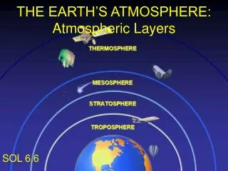
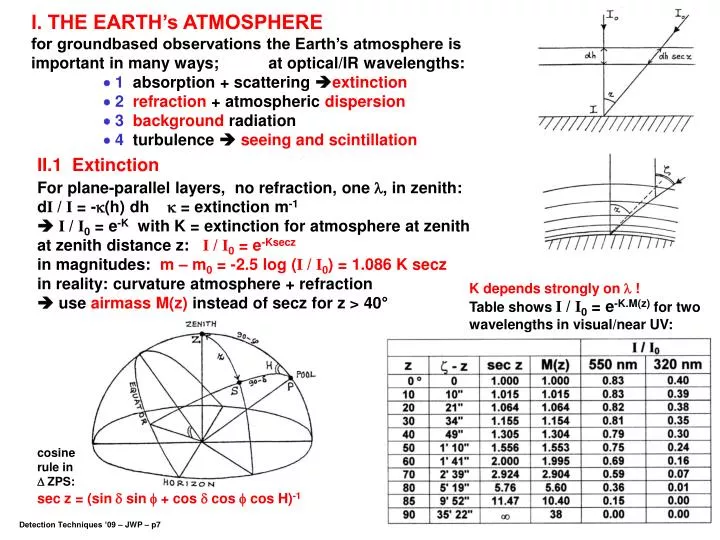
cosine rule in D ZPS: sec z = (sin d sin f + cos d cos f cos H)-1 I. THE EARTH’s ATMOSPHERE for groundbased observations the Earth’s atmosphere is important in many ways; at optical/IR wavelengths: 1 absorption + scattering extinction 2refraction + atmospheric dispersion 3background radiation 4turbulence seeing and scintillation II.1 Extinction For plane-parallel layers, no refraction, one l, in zenith: dI / I = -k(h) dh k = extinction m-1 I / I0 = e-K with K = extinction for atmosphere at zenith at zenith distance z: I / I0 = e-Ksecz in magnitudes: m – m0 = -2.5 log (I / I0) = 1.086 K secz in reality: curvature atmosphere + refraction use airmass M(z) instead of secz for z > 40° K depends strongly on l ! Table shows I / I0 = e-K.M(z) for two wavelengths in visual/near UV: Detection Techniques ’09 – JWP – p7
limit for groundbased photometry Sun no longer detectable Main extinction contributions in the classical optical region (l ~ 300-1000 nm): 1) Rayleigh scattering by air molecules; l –4 2) Absorption by O3; strong l-dependence especially in near-UV 3) Scattering by aerosol particles; not very l-dependent Local variations in aerosol contributions are very large, even between different observatories at same elevation: The very steep cutoff at ~ 300 nm is partly due to l –4 of Rayleigh scattering, but the O3 absorption dominates: Strong O3 absorption is remarkable in view of small O3 amount: 3 mm at standard (T,P); equivalent of whole atmosphere is 8.5 km. For l < 230 nm O3 opacity drops, but atmosphere remains opaque because of Rayleigh scatt. + absorptions by O2 + N2. from H. Tüg, thesis, 1978 Detection Techniques ’09 – JWP – p8
mm infrared extinction is dominated by molecular absorptions, mostly of H2O and CO2 observations are only possible in a number of ‘windows’, designated by I, J, K, L, M, N, Q H2O absorption depends strongly on humidity highly variable ! requires high and very dry observatory sites Detection Techniques ’09 – JWP – p9
In the IR strong H2O absorption causes deviations from the standard Edlén formula (Mathar, 2004) Red: standard (n-1) formula Blue: including effect of H2O II.2 Refraction and atmospheric dispersion Zenith distance as observed from the ground is always < z outside atmosphere. For precise calculation of refraction one needs: curved atmosphere geometryrefractive index along line of sight complex: depends on P,T and composition (humidity !) as function of height In the visual a good approximation till z = 75° is: (z – z)550 = (60.4“).tan z - (0.064“). tan3z (l = 550 nm, P= 1013 bar, 0° C) Refractive index n is function of l dispersion image becomes spectrum (z – z) l differs by factor (nl –1)/(n0 –1) with respect to (z – z)550 Typical values in visual l –range: l(nm)300 400 500 600 800(nl –1)/(n0 –1)1.047 1.014 1.001 0.995 0.989 nair at 550 nm: 1.000293 (P= 1013 bar, 0° C) Detection Techniques ’09 – JWP – p10
without Moon, Zodiacal light Q. : why this change ? Q. : can you explain this difference ? • • II.3 Atmospheric background radiation It is sometimes convenient to express astronomical surface brightness in ‘S10 units’: S10 = equivalent number of 10th magnitude stars per (deg)2 Main contributions to atmospheric sky background at dark site: • twilight at sunset/sunrise • moonlight • airglow and aurora • thermal emission twilight sky brightness in zenith at l = 550 nm (in S10 and mag/(arcsec)2) between sunset and ‘end of astronomical twilight’ (hSUN = -18 °) : Ex.: resolution human eye: ~1arcmin at hSUN =0° sky brightness per res. element is –1.7mag, i.e. brighter than brightest stars moonlight average brightness of moonlight as a function of lunar phase, in mag/(arcsec)2 for V and B Detection Techniques ’09 – JWP – p11
airglow and aurora airglow (nightglow) is line-emission that arises in the upper atmosphere from photo-ionization/dissociation and photo-chemical reactions driven by UV sunlight most reactions involve O/O2/O3, N/N2, Na, H2O, OH: nightglow is strongly variable, both spatially and in time Ex.:all-sky 6300 Å maps made at Haleakala (Hawaii), 15min intervals figures from Roach & Gordon: ‘The Light of the Night Sky’ (1973) Detection Techniques ’09 – JWP – p12
tables from Roach & Gordon: ‘The Light of the Night Sky’ (1973) many different reactions contribute to nightglow: nightglow lines can be very bright (OI 5577 Å, OH bands in near-IR ) stay away from them ! Detection Techniques ’09 – JWP – p13
near-IR nightglow is dominated by OH emission (rotation-vibration bands) a forest of emission lines, but between these lines the sky is very dark and the lines are narrow higher spectral resolution (R > 104) helps ! atmospheric radiation quantities are frequently expressed in Rayleigh units: at given l 1 R 4p . (surface brightness B) with B in units of (106 quanta) . cm-2. s-1.sterad-1 relation to S10: 1 R.Å-1 = 227 S10 (vis) example of OH lines in H-band: Table + fig. From Maihara et al. PASP 105, 940,1993 Detection Techniques ’09 – JWP – p14
Principal upper atmosphere emissions (Roach & Gordon 1973) aurorais transient emission driven by high-energy particles from the Sun mostly a polar phenomenon usually unimportant for observatories at latitudes < 40° when active, aurora can be much brighter than nightglow most prominent auroral lines: OI 5577 Å, 6300 Å, Ha 6563 Å Detection Techniques ’09 – JWP – p15
thermal atmospheric emission for l > 2.5 mm thermal radiation from the atmosphere becomes the dominant sky background (hence: the ‘thermal infrared’) RADIANCE W cm-2 sr-1m-1 Teff(atmosphere) 250 K peak at l 12 mm, but note: atmosphere is not a black body ! Sea level Kirchhoff: in thermal equilibrium emissivity = absorptivity IR sky emissivity is ‘mirror image’ of IR atmospheric transmission curve this hits us twice: katm. high large fraction of source photons removed and high sky background consequence for ground-based observations in the thermal IR: nearly all astronomical sources are very faint w.r.t. sky background Detection Techniques ’09 – JWP – p16
Ex.:a Lyr at l = 20 m: Fn = 12 Jy Fl = 5.8 x10⁻¹⁴ W.m-2.m-1 this wasoutside atmosphere on the ground: 1.6 x10⁻¹⁴ W.m-2.m-1 sky radiance: 10-5 W.cm-2.sr-1.m-1 = 2.4 x10⁻¹²W.m-2.m-1.(arcsec) –2 so if PSF = 1arcsec (diffraction-limited 8-m telescope at 20 m): Fsky = 150 x F(a Lyr)120 mJy source (m20m = 5mag): Fsky= 15000 x Fsource ! solution: differential measurementsby means of ‘chopping + nodding’ Example: FRAME TYPE 1: SKY+STAR no chop-subtraction star invisible w.r.t. high sky level FRAME TYPE 2: STAR ONLY sky removed by subtracting chopped/nodded frames VLT + VISIR Q-band spectroscopy medium resolution: R 1500 A B nod-pos. 1 6” A’ B’ NB: all ‘raw’ data, no flat-fielding slit length 32.5” nod-pos. 2 18.2 m more noisy horizontal bands: drop in S/N at strong sky line clusters 18.6 - - + 3 chopped/nodded spectra of star HD4128 (F18m = 25 Jy) strong absoptions due to sky lines, but good S/N (> 100) in clean windows Detection Techniques ’09 – JWP – p17
zodiacal light is strongly concentrated towards Sun and ecliptic plane: in the range l = 3-70 mthermal emission from zodiacal dust dominates the sky brightness Gegenschein at180° Note scale: 1 MJy/sterad = 2.35x10⁻⁵ Jy/arcsec2 ISO data, Leinert et al. A&A 393,1073, 2002 zodiacal light in the visual: scattering note surface brightness values in S10 l (m) compare with backgr. of stars + galaxies: comparison with sky background outside atmosphere outside atmosphere the optical/IR sky brightness is determined by: •dust particles in inner solar system zodiacal light• integrated light of faint stars and galaxies Detection Techniques ’09 – JWP – p18
II.4 Atmospheric turbulence turbulence is caused by temperature fluctuations in the convectively unstable troposphere (h < 10 km) thermal conductivity of air is low DT can live long DP is smoothed out very quickly (sound velocity !) a) turbulence cells have (DT, Dr) w.r.t. environment, but DP = 0 b) once formed, these cells can live rather long (> 1 s) the lightpath is influenced by Dr because (n-1) r turbulence cells work as weak positive/negative lenses that float with wind velocity through the line of sight causing 2 effects: fluctuations in direction ‘seeing’ fluctuations in brightness ‘scintillation’ apply ideal gas law (index 0 for ambient quantities outside cell): (n-1)/(n0 –1) = r / r0 = (PT0) / (P0T), P = P0 Dn = -(n0-1).(T0/T2).DT at sea level: T T0 300K, n0 = 1.000293 (l = 550 nm) Dn 10-6 .DT at altitude h: (nh-1) = e-h/H .(n0-1) with H = scale height atmosphere 8.5 km Dn = -10-6 .e-h/H .DTDT 0.1-1 K, h < 10 km cells have Dn 10-6–10-7 direction changes in range 0.1-1 arcsec Detection Techniques ’09 – JWP – p19
flat wavefront scintillation: DI h.e-h/H seeing: Df e-h/H L” = L –2h.Df very simple model for optical effects of turbulence cell assume: atmosphere is isothermal, in hydrostatic equilibrium take turbulence cell at height h, with diameter L and n = n0+Dn in figure: Dn > 0 (DT < 0) wavefront retarded inside cell observations confirm this: turbulence in lower layers has highest weight for seeing (ground layer and dome seeing !) for small h and typical DT 1°: Df = 2x10⁻⁶ rad = 0.4” Dtel. L :at any time only 1 cell in beam PSFtelescope unaffected, but whole image shifts Dtel > L : image is smeared into seeing disc without seeing a diffraction-limited telescope with aperture D >L has PSF-diam. d = 1.2 l/D (D= 10 m, l = 0.5 m d = 0.01”) with seeing: image becomes blob of rapidly moving ‘speckles’ with overall diam. Df regardless of telescope diam. (diam. speckles:1.2 l/D) a)direction changes: seeing L’ = L[n0/(n0+Dn)] Df = 2(L-L’)/L = = 2Dn / (n0+Dn) 2Dn = -2x10⁻⁶. DT .e-h/Hthis function peaks at h = 0 Detection Techniques ’09 – JWP – p20
b) intensity changes: scintillation DI/I on the ground is proportional to h. Df, i.e. h.e-h/H this function has maximum at h = H = 8.5 km scintillation comes mostly from high layers seeing and scintillation are usually uncorrelated also these results are confirmed by observations: •a typical cell with 10 cm at h=8.5 km has angular diam. 2” planets don’t scintillate ( Mars: ~5-15”,Jupiter: ~40-50”, Venus: 15-60”) •the seeing and scintillation fluctiations are usually uncorrelated scintillation amplitude + frequency for small telescope apertures: scintillation amplitudeDI/I - drops below 100 Hz - decreases strongly with Dtel this fits with typical cell sizes (5-25 cm) and wind speeds at 8-10 km (~100 km/h) DI/I is largest for D turbulence cell (e.g. human eye !) Dtel > 1m scintillation becomes negligible (averages out over many cells) Detection Techniques ’09 – JWP – p21
more realistic description of wavefront distortions by atmospheric turbulence Lit.: Beckers: Ann. Rev. A&A Vol.31, 13, 1993 a proper description should take into account: •atmospheric turbulence in reality is a 3-D field of cells with a distribution of cell sizes and temperature variations • the atmosphere is in hydrostatic equilibrium, but not isothermal i.e. T = T(h) NB: from now on we concentrate on seeing, as scintillation for large telescopes is unimportant NB: ongoing dispute about Lu ! for Paranal: median Lu 22 m Kolmogorov (1941): in a turbulent gas flow the kinetic energy of the turbulence eddies with spatial frequencies f is f-5/3 this power law holds between scale Lu (‘outer scale of turbulence’ = scale at which turbulence is generated) and Ll (lower scale, where turbulence dissipates by viscosity very small) on the basis of Kolmogorov turbulence Tatarski (1961) developed the theory that is commonly used in astronomical seeing models most important parameters: DT(Dr) <|T(r +Dr) –T(r)|2> (in K2) = variance in T for two points Dr apart for Kolmogorov turbulence: DT(|Dr|) = CT2 .|Dr|2/3 (CT2 = ‘structure constant of T-variations’) DT DrDn structure function for n: Dn(|Dr|) = Cn2 .|Dr|2/3 where Cn = 7.8x10⁻⁵ .(P/T2). CT (at l = 0.5 m, P in mbar) Detection Techniques ’09 – JWP – p22
fluctuations in n cause fluctuations in phase and amplitude (amplitude scintillation: can be neglected for large telescopes) • integrated effect of all phase fluctuations along light path through atmosphere is equivalent with ‘phase screen’ in front of observer that makes originally flat wavefronts corrugated for Kolmogorov turbulence the phase ‘structure function’ at the entrance of the telescope is: Df(Dx) = <|f(x +Dx) –f(x)|2> = 6.88 r0-5/3. Dx5/3 (in rad2) with r0 = the coherence length (= ‘Fried parameter’) : r0(l, z) = [0.423 .(2p/l)2.sec z . Cn2(h)dh]-3/5= 0.185 .l6/5 . cos3/5z . [ Cn2(h)dh]-3/5 convention: unless stated otherwise r0 r0(l = 0.5 m, z = 0°) other l: scale l6/5 r0 is related to the ‘isoplanatic angle’ 0=radius of sky area where wavefronts can be considered as coherent (flat) 0 = 0.341r0/H (H = average distance of seeing layer) seeing from thick layers: H = secz. { h5/3.Cn2dh / Cn2dh }3/5 0 + wind velocity characteristic timescale:t0 = 0.341r0/Vwind r0 10 cm (r0 size of average seeing cell) typical seeing-dominated PSF (for r0 < Dtel.): d (FWHM) l/r0 1” if seeing layer at h=10 km 0 0.7” with Vwind = 10 m/s: t0 = 0.003 s, or f0 = 300 Hz typical values at l = 0.5 m : Detection Techniques ’09 – JWP – p23
turbulence often occurs in 3 domains: incoming flat wavefront boundary troposphere-stratosphere wind-shear turbulence (jet streams !) this limits best seeing at best sites (when turb. at h2 and h3 negligible): r0 20 cm l/r0 0.5”, 0(h1) 1.4” high Vwind (~100 km/h) t0 2 ms h1=10-12 km r0 (h1) 0(h1) corrugated wavefront h ‘planetary boundary layer’ turbulence from convection driven by daily solar heating if r0 (h2) = r0 (h1) 0 (h2) = 10x0 (h1) lower wind speeds t0 5 ms h2 1km r0 (h2) 0 (h2) h3 < 30 m surface layer turbulence from wind-surface interaction (+ man-made !) small h 0 (h3) up to few arcmin t0 10 ms r0 (h3), 0 (h3) NB: if there is turbulence in the lowest layers this usually dominates seeing because (n-1)h rh e-h/H Detection Techniques ’09 – JWP – p24
II: SYSTEM CALIBRATION: SETTING UP A SYSTEM OF SPECTROPHOTOMETRIC STANDARDS the Walraven 5-channel photometer was one of the few simultaneous multi-band photometers that operated in the period ~1960-’90 other example: Strömgren (uvby) photometers example: the standards for the Walraven (V,B,L,U,W) photometric system big advantage of simultaneity: extinction variations are ~ ‘gray’ high precision in colours NOTE: 0.01m colour errors significant and correlated errors in (IS reddening,Teff, logg, [Fe/H], age) • calibration ‘from scratch’ was done twice: • by Th.Walraven during start of observations at the Leiden Southern Station in S.-Africa • 1979 by J.Lub + J.W.Pel after move of telescope +instrument to ESO,Chile because of: •different atmosphere+elevation • new photomultipliers •new telescope mirror coatings Lit.: Pel, J.W., Lub, J., in ‘The Future of Photometric, Spectrophotometric and Polarimetric Standardization’ ASP Conf. Ser. #364, p.63, Ed. C.Sterken, 2007 Detection Techniques ’09 – JWP – p48
1) select ~ 20 suitable stars in ring around the sky close to Dec= fgeogr 2) observe star pairs when D(secz) ~ 0 within Dt < 10 min 1st approx. of extinction coeff. are OK for accurate D(mag)i in all channels, detector gain drifts drop out due to small Dt 3)repeat pair observations many times and take averages accuracy of D(mag)i per pair: ~0.001mag 4) make least-squares solution for whole network of pair differences residuals now <0.0005mag ! 5) check residuals for systematics (dependence on brightness, colour, position, time….) 6) all magnitudedifferences (flux ratios) now accurately known, but zeropoints still arbitrary define one primary standard as zeropoint in this case: HD144470 (O-star so SED BB ) VW (144470) chosen to match VUBV, all four Walraven colour indices defined as zero 7) standards can now be used for determination of extinction coeff. + instrumental zeropoints for all nights connect all secondary standards to the ‘ring standards’ 8) connect the whole set of standards to stars with absolute flux calibrations this gives relations [(VBLUW) magnitudes physical flux densities] strategy: Detection Techniques ’09 – JWP – p49
9) external verification the ‘ring solution’ method produced standards with high internal precision, but there might still be hidden systematic errors for checks with external data, a set of ~2000 stars with multiple high-quality VBLUW obs. was compared with data in the Johnson (U B V), Strömgren (u v b y) and Geneva (U B1 B2 V1 V2 G) systems comparison was possible for two transformable quantities: VW VJ VG ySand (V-B)W (B-V)J (B2-V1)G (b-y)S result: a) large scatter and systematic RA-dependent differences in comparison with VJ,(B-V)J no surprise: UBV photometry is very inhomogeneousb) systematic RA-trends in comparison with VG, (B2-V1)G very unexpected !c) smallest scatter and no systematics in comparison with yS, (b-y)S Walraven and Strömgren systems OK ! Detection Techniques ’09 – JWP – p50
additional checks with data from space 1) comparison between VW and HIPPARCOS Hp magnitudes: no systematic trends as a function of (colour, RA, DEC) both photometric systems are ‘flat’ to level of 0.001 mag 2) comparison between WW and IUE spectrophotometry for SN 1987a (LMC) excellent agreement Note: this now includes the absolute flux calibration, for l close to the UV atmospheric cut-off ! Detection Techniques ’09 – JWP – 51