Recap (I)

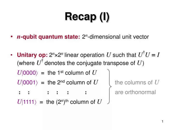
1. Recap (I) • n-qubit quantum state:2n-dimensional unit vector • Unitary op: 2n2n linear operation U such that U†U=I(where U† denotes the conjugate transpose of U) U0000 =the 1st column of U U0001 =the 2nd column of U the columns of U : : : : : :are orthonormal U1111 =the (2n)th column of U

2. “old” notation “new” notation a a AND gate a Λb Λ a Λb b b a NOT gate a a  a Classical (boolean logic) gates Note: an OR gate can be simulated by one AND gate and three NOT gates (since a Vb= (a Λb))

3. 1 Λ Λ 1 Λ Λ 0 1 Λ Λ Λ 1 1  Λ 0    0 Λ Λ 1 0 Λ  Λ 1 1 Λ  data flow 0 1 0 1 1 1 0 0 1 1 Models of computation Classical circuits: Quantum circuits:

4. Multiplication problem Input: two n-bit numbers (e.g. 101 and 111) • “Grade school” algorithm costs O(n2) • Best currently-known classical algorithm costs O(nlogn loglogn) • Best currently-known quantum method: same Output: their product (e.g. 100011)

5. Factoring problem Input: an n-bit number (e.g. 100011) • Trial division costs  2n/2 • Best currently-known classical algorithm costs  2n⅓ • Hardness of factoring is the basis of the security of many cryptosystems (e.g. RSA) • Shor’s quantum algorithm costs  n2 • Implementation would break RSA and many other cryptosystems Output: their product (e.g. 101, 111)

6. Recap: states, unitary ops, measurements • Classical computations as circuits • Simulating classical circuits with quantum circuits • Simulating quantum circuits with classical circuits • Simple quantum algorithms in the query scenario

7. a a b b c (a Λb)c  Toffoli gate (Sometimes called a “controlled-controlled-NOT” gate) Matrix representation: In the computational basis, it negates the third qubit iff the first two qubits are both 0

8. Quantum simulation of classical a a 1 1 AND gates NOT gates b b 1 1 garbage a a Λb a 0 Theorem: a classical circuit of size s can be simulated by a quantum circuit of size O(s) Idea: using Toffoli gates, one can simulate: This garbage will have to be reckoned with later on …

9. 0 H random bit 0 isolate this qubit 0 H use in place of coin flip Simulating probabilistic algorithms Since quantum gates can simulate AND and NOT, the outstanding issue is how to simulate randomness To simulate “coin flips”, one can use the circuit: It can also be done without intermediate measurements: Exercise: prove that this works

10. Recap: states, unitary ops, measurements • Classical computations as circuits • Simulating classical circuits with quantum circuits • Simulating quantum circuits with classical circuits • Simple quantum algorithms in the query scenario

11. Classical simulation of quantum Theorem: a quantum circuit of size s acting on n qubits can be simulated by a classical circuit of size O(sn22n) =O(2cn) Idea: to simulate an n-qubit state, use an array of size 2n containing values of all 2n amplitudes within precision 2−n Can adjust this state vector whenever a unitary operation is performed at cost O(n22n) From the final amplitudes, can determine how to set each output bit Exercise: show how to do the simulation using only a polynomial amount of space (memory)

12. Some complexity classes • P (polynomial time):problems solved by O(nc)-size classical circuits (decision problems and uniform circuit families) • BPP (bounded error probabilistic polynomial time): problems solved by O(nc)-size probabilistic circuits that err with probability  ¼ • BQP (bounded error quantum polynomial time):problems solved by O(nc)-size quantum circuits that err with probability  ¼ • EXP (exponential time): problems solved by O(2nc)-size circuits.

13. EXP PSPACE BQP BPP P Summary of basic containments P BPP  BQP  PSPACE  EXP This picture will be fleshed out more later on

14. Recap: states, unitary ops, measurements • Classical computations as circuits • Simulating classical circuits with quantum circuits • Simulating quantum circuits with classical circuits • Simple quantum algorithms in the query scenario

15. x f f(x) Answer: d +1 Query scenario Input: a function f, given as a black box (a.k.a. oracle) Goal: determine some information about f making as few queries to f (and other operations) as possible Example: polynomial interpolation Let:f(x) =c0+c1x+c2 x2+ ... + cd xd Goal: determine c0 , c1 , c2 ,... , cd Question: How many f-queries does one require for this?

16. Deutsch’s problem f Let f : {0,1}  {0,1} There are four possibilities: Goal: determine whether or not f(0)=f(1) (i.e. f(0)  f(1)) Any classical method requires two queries What about a quantum method?

17. alternate notation: A classical algorithm: (still requires 2 queries) 0 1 f f f f(0)  f(1) 0 Reversible black box for f a a Uf b bf(a) 2 queries + 1 auxiliary operation

18. 2 3 1 f Quantum algorithm for Deutsch H H f(0)  f(1) 0 H 1 1 query + 4 auxiliary operations How does this algorithm work? Each of the three H operations can be seen as playing a different role ...

19. H H 0 H 1 f f x (–1)f(x)x NOT with eigenvalue –1 Iwith eigenvalue +1 0 –1 0 –1 Quantum algorithm (1) 2 3 1 1. Creates the state 0 –1, which is an eigenvector of This causes f to induce a phase shift of (–1)f(x) to x

20. (–1)f(0)0 +(–1)f(1)1 0 H f 0 –1 0 –1 Quantum algorithm (2) 2. Causes f to be queried in superposition (at 0 + 1) (0 +1) (0 –1)

21. H (0 +1) 0 H (0 –1) 1 Quantum algorithm (3) 3. Distinguishes between (0 +1) and (0 –1)

22. 2 3 H H f(0)  f(1) 0 1 H 1 f Summary of Deutsch’s algorithm Makes only one query, whereas two are needed classically extracts phase differences from (–1)f(0)0 +(–1)f(1)1 produces superpositions of inputs to f : 0 + 1 constructs eigenvector so f-queries induce phases: x (–1)f(x)x

23. Source of slides Introduction to Quantum Information ProcessingCS 467 / CS 667Phys 667 / Phys 767C&O 481 / C&O 681 Richard Cleve DC 653 cleve@cs.uwaterloo.ca Lecture 3 (2005)

24. Taught in 2007