Download

1 / 8
160 likes | 469 Views
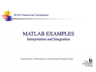
MATLAB EXAMPLES Initial-value problems. 58:110 Computer-Aided Engineering Spring 2005. Department of Mechanical and industrial engineering January 2005. Some useful functions. IVP.

E N D
MATLAB EXAMPLESInitial-value problems 58:110 Computer-Aided Engineering Spring 2005 Department of Mechanical and industrial engineering January 2005
IVP The initial value problems for 1st order differential equation are defined by the following standard form: • Example: The exact solution is: In the following slides, we will try to solve this problem by Euler and Runge-Kutta methods in MATLAB. The ODE function was defined as M-file (ex1_odefun.m): % IVP function for EX1 function xdot=ex1_odefun(t,x) xdot=x+1;
IVP –Euler method Use Euler method to solve the IVP example, step size sets to 0.01. Write the M-file as follows (ivp-euler.ex1.m): % IVP solution - Euler method % example 1: x'=x+1, x(0)=0, solve x(1) % the range of t [a,b] a=0.0; b=1.0; % the initial value of x x=0.0; %the number of steps n=100; %set the matrix x0=zeros(n,1); % set the step size h=(b-a)/100; %set the initial value of t t=a; for k=1:n % Record the values of x in each step x=x+h*ex1_odefun(t,x); x0(k)=x; t=t+h; end %the final result of x x0(100) • Run this M-file: >> ivp_euler_ex1 • ans = • 1.7048
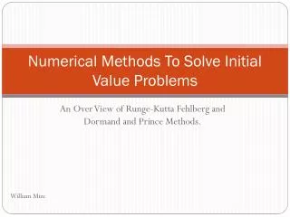
IVP –Runge-Kutta method To use Runge-Kutta method, here we only try ode23 and ode45 (step size =0.1): >> tspan=linspace(0,1,11); >> x0=[0;0]; >> [t,x]=ode23(@ex1_odefun,tspan,x0); >> x(11) ans = 1.7182 >> [t,x]=ode45(@ex1_odefun,tspan,x0); >> x(11) ans = 1.7183 The results show the higher order solver ode45 got more accurate result than ode23 and Euler method.
IVP - Plot To show the accuracy of different methods, we need plot the solution together, the following M-file is for plotting the results of exact, Euler and 4th Runge-Kutta methods (ivp-plot_ex1.m): % IVP solution - plot % example 1 x'=x+1 % the range of t [a,b] a=0.0; b=1.0; % the initial value of x x=0.0; %the number of steps n=10; %set the matrix x1=zeros(n,1); %the step size h=(b-a)/10; %set the initial value of t t=a; %Euler method - Iterations for k=1:n+1 % Record the values of x in each step x1(k)=x; x=x+h*ex1_odefun(t,x); t=t+h; end %plot the results t=linspace(0,1,11); %Runge-Kutta method rx0=[0;0]; [t,x2]=ode45(@ex1_odefun,t,rx0); %exact solution x0=exp(t)-1; plot(t,x0,t,x1,'.',t,x2,'o') xlabel('t') ylabel('x')
IVP - Plot • The following figures show the results by different step size h. The solid line is the exact solution, the solid dots represent the result of Euler method, the circles represents the results of 4th order Runge-Kutta method. h = 0.1 h = 0.01
IVP-Summary Compare the results of different methods (all keep 4 digits after the radix point) in the following table (x(1)):