Download
1 / 40
400 likes | 524 Views
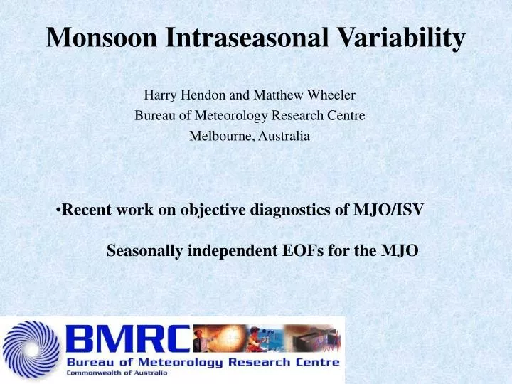
Monsoon Intraseasonal Variability. Recent work on objective diagnostics of MJO/ISV Seasonally independent EOFs for the MJO. Harry Hendon and Matthew Wheeler Bureau of Meteorology Research Centre Melbourne, Australia. Issues to be addressed :

E N D
Monsoon Intraseasonal Variability • Recent work on objective diagnostics of MJO/ISV • Seasonally independent EOFs for the MJO Harry Hendon and Matthew Wheeler Bureau of Meteorology Research Centre Melbourne, Australia
Issues to be addressed: • Does near-equatorial, eastward propagating, convectively-coupled, baroclinic MJO occur year-round? • Is the MJO properly defined in Northern Hemisphere Summer? • Is there poleward propagating ISV independent of MJO? • (or, how much of the poleward propagating ISV in the monsoon can be attributed to the MJO?) • Devise an objective definition for MJO • Document annual/interannual variation in propagation/strength/off-euatorial behavior.
Seasonally independent EOFs for the MJO Require a standard metric of the MJO that: 1) captures its salient properties 2) is easy to compute 3) can be computed in real time for forecast and monitoring application 4) provides insight into dynamics/physics
Salient properties MJO baroclinic disturbance, coupled with convection, eastward along the equator as originally depicted by MJ 1972 But, MJO exhibits strong annual variation in strength and especially in off-equatorial structure/propagation Madden and Julian (1972)
Ingredients of MJO diagnostic Use U850, U200, OLRto capture convective/baroclinic structure, Average about equator (15N-15S) to focus on zonal propagation, (i) Removal of seasonal cycle (ii) Removal of variability associated with index of ENSO (iii) Removal of mean of previous 120-days (all these steps can be performed in real-time) Compute EOFs in order to objectively extract dominant mode Prior to EOF, normalize each field by globally-averaged variance.
U850 U200 OLR %Variance explained by each EOF
Project raw anomaly data onto the EOFs Spatial projection onto “MJO structure” effectively discriminates to MJO periods ¼ cycle Phase lag EOFs are temporally in quadrature, thus describing a zonally propagating disturbance Coh**2
What’s the nature of ISV variability associated with the MJO and independent of MJO? Define MJO part by multiple linear regression onto principal components : OLRMJO(x,y,t) = a(x,y) + b(x,y)RMM1(t) + c(x,y)RMM2(t) N.B. Regression coefficients are a function of season Then define an MJO part, and a residual, OLRANOM=OLRMJO+OLRRESIDUAL
MJO part “MJO” Total RESIDUAL Leading pair of EOFs captures all of the eastward propagating variance
“MJO” OLR variance DJFM JJAS
DJF JJA total MJO residual
May-Oct -30 Lag d Regression OLR (shade), U850 onto MJO PCs +30 Nov-Apr Behavior along eq is independent of a season
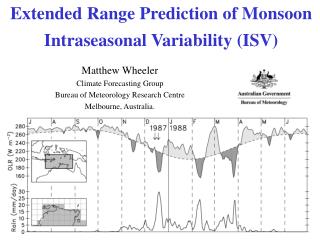
Dates defined using Darwin zonal wind (Drosdowsky 1996). Kerala dates defined using rainfall by IMD (e.g., Joseph et al. 1994). W Pacific W Pacific Maritime Continent Maritime Continent Africa Africa Indian Indian
Total May-Oct North-south propagation 30° in 20 days 2-d spectrum in meridional direction 20°S-40°N 80-90°E Zero-pad in meridional direction to give equivalent 90°S-90°N periodic domain i.e., Wave 1 has 20000km wavelength “MJO” RESIDUAL
Total Nov-Apr 40°S-20°N data only 80-90°E Zero-pad in meridional direction to give equivalent 90°S-90°N periodic domain i.e., wave1=10000km half-wavelength “MJO” RESIDUAL
Looking another way: Lagged regressions with OLR in base region “MJO” DJFM: BP=80-90°E,5-10°S JJAS: BP=80-90°E,5-10°N RESIDUAL Regressed OLR plotted, based on a 1 standard deviation anomaly in the predictor
RESIDUAL JJAS regressed OLR and 850hPa winds Base Point = 80-90°E, 5-10°N Primarily northward propagation Some westward
Conclusions MJO exists year-round, with constant near-equatorial structure. MJO accounts for ~1/2 poleward propagating ISV in monoon Independent northward propagation has higher frequency and shorter meridional and zonal scales Implication: mechanism of equatorial propagation is independent of poleward propagation But, is mechanism of poleward propagation the same for the MJO as for the independent component?
US CLIVAR: MJO WORKING GROUP Duane Waliser, co-chair Wanqui Wang Ken Sperber, co-chair Chidong Zhang Siegfried Schubert 2-Yr Lifetime Mitch Moncrieff Klaus Weickmann April 2006-> Eric Maloney Bin Wang Leo Donner F. Vitart, S. Woolnough*, H. Hendon*, M. Wheeler*, W. Higgins, J. Gottschalck, W. Stern * International CLIVAR Support http://www.usclivar.org/Organization/MJO_WG.html • Terms of Reference • Develop a set of metrics to assess MJO simulation and forecast skill. • Coordinate model simulation and prediction experiments to better understand and improve MJO • Raise awareness of utility of MJO forecasts in the context of the seamless suite of predictions. • Coordinate MJO-related activities between national and international agencies
….compared to variance of “RESIDUAL” field (i.e., variance of what’s left when “MJO” part is removed from original anomaly field) DJFM 10 times the contour interval! JJAS
15°S–15°N averaged OLR Annual cycle of MJO Variance
Kemball-Cook and Wang’s composite of the May-June “BISO” based on OLR in the box poleward and eastward along equator also Lawrence and Webster
Diagnostics of MJO/ISV Motivation: continued poor representation of MJO/ISV in forecast/climate models importance for monsoon variability/prediction Provide quantifiable/consistent measures Elucidate mechanisms/physics Compare simulations/forecasts with observations Applicable in realtime to make/assess forecasts
Space-time spectral analysis • Quantifies space and time scales of organized/propagating behavior • Long history for identification wave modes of tropical intraseasonal variability Kelvin waves, Rossby-gravity waves, MJO • Normalized spectra (WK99) emphasized prominent role of wave modes for organization of tropical convection • revisit WK99: objective/physical estimation of background spectrum (hopefully conclusions don’t depend on definition of background) space-time coherence spectrum OLR/zonal wind
Ratio Spectrum/Background Symmetric OLR 15N-15S Only obvious peak is MJO Wheeler & Kiladis 1999
Background Spectrum WK99 estimated background spectrum by ad-hoc smoothing in wavenumber and frequency Alternate approach: Assume background variability can be modeled as 1st order auto-regressive process (Gilman et al. 1963): X(n)=pX(n-1) +noise p is the lag-1 autocorrelation, obtain by inverse Fourier transform of power spectrum The equivalent auto correlation function is cor(T)=pT where T is lag. Equivalent power spectrum can be obtained by inverse transform of the correlation function (or approximate discrete formula provided by Gillman et al) E(f)~1/(const+f2) power spectrum of “red noise” E(f) is computed for each zonal wavenumber and normalized to have the same power as the actual spectrum for that wavenumber.
OLR 10N-10S equivalent “red” spectrum smth background WK99
Quantify “redness” of background For a first order auto regressive process, the discrete autocorrelation function is cor(T)=pT Decorrelation time defined as the time for the correlation to drop to a value of e-1 : Td=-(lnp)-1
Decorrelation time(d) of background red spectrum 10N-10s decorrelation time (d)
Symmetric OLR 10N-10S Shading is signal: percentage of power that stands above red background WK99: Shading is ratio of actual spectrum to background spectrum
OLR 10N-10S 20 m/s U850 10N-10S
Space-time Coherence Spectrum effectively correlation as function of wavenumber and frequency The phase lag . where Q is imaginary part (quad) of cross spectrum and P is real part (co)
Coherence OLR and U850 Coh**2: direct measure of interaction of convection with large-scale circulation doesn’t rely on definition of background
OLR/U850 OLR/U150 OLR/U50
MMF (“super parameterization”) CAM (Zhang and McFarlane) Precip MMF U850 CAM
Precip MMF (NCAR CAM3) “Super parameterization” U850