Download
1 / 43
430 likes | 456 Views
The Time Variation in Risk Appetite and Uncertainty. Geert Bekaert Columbia, NBER. Eric Engstrom Federal Reserve Board. Nancy Xu Boston College. The views expressed in this document do not necessarily reflect those of the Federal Reserve System, its Board of Governors, or staff.

E N D
The Time Variation in Risk Appetite and Uncertainty Geert Bekaert Columbia, NBER Eric Engstrom Federal Reserve Board Nancy Xu Boston College The views expressed in this document do not necessarily reflect those of the Federal Reserve System, its Board of Governors, or staff.
I. Introduction Three Recent Mood Swings “Financial markets have recently been alternating between “risk on” (when markets are in buoyant mood) and “risk off” (when they are anxious) with bewildering rapidity.” – The Economist, “Mood Swings”, Oct 2011 “A low VIX reading is usually seen as a sign of investor complacency.” – The Economist, “The markets are quiet. Too quiet?”, May 2017 “Fear that inflationary pressures would cause bond yields to rise and central banks to push up interest rates translates into the sharp jump in the VIX in early February.” – The Economist, “The markets still have plenty to fret about”, Feb 2018
I. Introduction Motivation • Changes in risk appetite: Important determinant of assetprices • Behavioralfinance • (e.g. Baker & Wurgler,2006) • Structural dynamic asset pricing • (e.g. Campbell & Cochrane, 1999 + manyvariants) • Reduced-form asset pricing and optionpricing • (e.g. Bakshi & Wu 2010; Broadie, Chernov & Johannes,2007) • Monetary policy transmissionchannel • (e.g., Adrian & Shin, 2009; Bekaert, Hoerova & Lo Duca,2013) • Internationalfinance • (e.g. Miranda-Agrippino & Rey, 2015; Xu,2017) • No agreement on how to measure aggregate risk aversion
I. IntroductionModeling Risk Aversion • Impossible to define a model – free measure: Risk premium asset i Beta asset i “price of risk” [CAPM] risk aversion market variance [consumption CAPM; power utility] consumption growth variance risk aversion • Risk aversion ≠ price of risk; our definition: risk appetite = inverse of risk aversion.(in contrast: Coudert and Gex (2008); Pflueger, Siriwardane and Sunderam (2018))
I. Introduction Our Measure of Time-Varying Risk Aversion (1) Controls for macroeconomic and cash flow uncertainty Digression: Relative new tractable model of heteroskedasticity and non-Gaussian dynamics (“BEGE”) (2) Helps consistently price major risky asset classes: • equities • corporate bonds (3) Depends implicitly on macro data, asset moments of equity and corporate bond returns; variances and option prices (4) Is easy to compute and measurable at high frequencies as it is spanned by observable financial information
II. The ModelModeling Risk Aversion - Introduction • Our approach: • Specify a utility framework to price risk assets • - generalization of Campbell and Cochrane’s habit framework • Define risk aversion as the RRA of the marginal investor • Define economic uncertainty as second moments of fundamentals • Model RA state variable to be imperfectly correlated with fundamentals
II. The ModelStep 1 - Macro Environment • Macro shocks: likely to be non-Gaussian and asymmetric, with time-varying volatilities (and higher moments) Hamilton (1990); Fagiolo, Napoletano & Roventini (2008); Gambetti, Pappa & Canova (2008); Addian, Boyarchenko & Giannone (2018); Bekaert and Engstrom (2017) • Filter uncertainty state variables from monthly industrial production growth, θt : (1) conditional mean growth shock (2) Gamma distribution “real” upside uncertainty (“good vol”) (3) “real” downside uncertainty (“bad vol”) (4) => “Bad Environment-Good Environment” dynamics: Bekaert & Engstrom (2017, JPE)
II. The ModelBEGE Framework: Examples of the BEGE Density 1) “Large” and equal pt and nt: Gaussian limit
II. The ModelBEGE Framework: Examples of the BEGE Density 2) “Small” but still equal pt and nt: excess kurtosis
II. The ModelBEGE Framework: Examples of the BEGE Density 3) Relatively large nt: negative skewness: “Bad Environment”
II. The ModelBEGE Framework: Examples of the BEGE Density 4) Relatively large pt: positive skewness “Good Environment”
II. The ModelBEGE Framework: Narcissism • We love the BEGE distribution…. • Many alternative applications: • Bekaert, Engstrom, Ermolov (2015, Journal of Econometrics): BEGE GARCH for stock returns • Bekaert and Engstrom (2017, JPE): consumption growth and the variance risk premium • Bekaert, Ermolov and Engstrom (2019): term structure, AS/AD macro shocks
II. The ModelBEGE Framework: Disclaimer …. but we have no affiliation with the Bee Gees
II. The ModelBEGE Framework: Moments and Dynamics • BEGE densities have simple affine expressions for all moments variance: (unscaled) skewness: Volatility dynamics: “good volatility” “bad volatility”
II. The ModelStep 2 – Preferences • Consider a period utility function in the HARA class: (7) Ct : consumption Qt = f(Ct): drives time variation in risk aversion Example: (Campbell and Cochrane, 1999) • The coefficient of relative risk aversion: (8) • The pricing kernel: (9)
II. The ModelStep 2 – Preferences Step 2 - Preferences Non-Gaussian Dynamic process: Shock Link to Structural Asset Pricing literature (e.g. Campbell & Cochrane
II. The ModelStep 3 – Cash Flow State Variables • CF variables for corporate bonds/equity (all in logs) • Corporate bond loss rate (default rate times 1 minus recovery rate) • Shows evidence of independent time-varying and skewed loss rate variance • “financial” uncertainty: lpt • Earnings growth • Dividend Payout Ratio • Consumption/earnings ratio Project on macro-state variables and shocks => Most processes show independent persistence, but uncertainty dynamics captured by macro and financial uncertainty
II. The ModelDynamic Asset Pricing Model – Model Solution • Matrix representation of the state variables: • Given pricing kernel, Γ – dynamics, price-coupon ratio (price-dividend ratio): (Quasi) Exponential affine in Yt • Log asset returns: • Closed-form solution: Time variation in risk premiums, physical conditional variances, risk-neutral conditional variance are exact Conditional Mean Shock Structure Approx. Error Upside macro uncertainty pt Downside macro uncertainty nt Financial uncertainty lpt Risk aversion qt functions of
III. The Identification and Estimation of Risk AversionEstimation Methodology - Philosophy • Step 1: Filter macroeconomic and financial uncertainties, {pt, nt, lpt} - do not use asset prices! • Step 2: Identify risk aversion, qt • Theory for an affine model: asset moments = exact functions of uncertainties (pre-determined) + risk aversion • qt should be spanned by asset prices and risk variables • => model qt as exact function of observable financial instruments • Unknown: spanning parameters in qt
III. The Identification and Estimation of Risk AversionEstimation Methodology - Empirical • Procedure: [eq=equity; cb=corporate bond] • Asset moments to be matched: risk premium (eq, cb), physical variance (eq, cb), risk-neutral variance (eq) • Spanning instruments: term spread, credit spread, 5-yr detrended earnings yield, realized variances (eq, cb), risk-neutral variance (eq) • Estimation: GMM; 1986/06 – 2015/02 • Advantages: • Risk aversion available at high frequencies • Disentangles risk aversion from uncertainty • Estimation procedure still imposes all model dynamics
Digression: Physical versus Risk Neutral Variances • Intuition: Risk Neutral versus Physical Variances ~ physical probabilities ~ “risk neutral” probabilities • Key empirical fact: qvar – pvar ≥ 0 (variance premium) Risk neutral = “utility-adjusted” (see Merton, 1969!) => transfer probability mass to high marginal utility states (“utility probabilities”) • VIX2 = average of option prices (Bakshi and Madan, 2000; Martin, 2018) • = variance risk premium + physical variance
III. The Identification and Estimation of Risk AversionEstimation Results – Step 1, Uncertainties
III. The Identification and Estimation of Risk AversionModel Estimation • GMM does not reject the model • Model Fit:
III. The Identification and Estimation of Risk AversionConditional Moment Decomposition • How important is the risk aversion state variable (qt) for asset prices? => Variance decomposition, βxCov(xt, Momt) / Var(Momt)
III. The Identification and Estimation of Risk AversionEstimation Results – Step 2, Risk Aversion Relative risk aversion, implied from risky asset markets
III. The Identification and Estimation of Risk AversionOur Indices • Risk aversion: • Economic uncertainty, reflected in financial instruments:
III. The Identification and Estimation of Risk AversionOur Indices
III. The Identification and Estimation of Risk AversionCorrelations with Extant Indices
III. The Identification and Estimation of Risk AversionPredictability Results – Risky Asset Returns • where: • “Mod”, Model-implied risk premiums – Variance Risk Premium
III. The Identification and Estimation of Risk AversionPredictability Results – Economic Growth Regression:
III. The Identification and Estimation of Risk AversionRisk Aversion Properties • Risk aversion: • countercyclical but mostly driven by “moodiness” • much less persistent than macro (habit) risk aversion • (see also Martin (2018)) • Risk aversion well proxied by the variance risk premium • (Bollerslev, Tauchen and Zhou, 2009; Bekaert and Hoerova, 2014) Recall: variance risk premium risk neutral variance physical (conditional) variance = – option prices projection models with realized variances; VIX
IV. Risk Aversion, Uncertainty and Monetary Policy • Does monetary policy affect risk appetite in financial markets? • (Excessive) risk-taking in asset management (Rajan, 2006) • Balance sheets of financial intermediaries (Adrian and Shin, 2010); MP affects broad liquidity and credit measures • Evidence for MP effects on risk appetite of banks (loan book; credit standards, . . . ) • Expansionary MP affects the stock market positively; see Thorbecke (1997) , Rigobon and Sack (2003, 2004), Bernanke and Kuttner (2005) • What about the VIX and monetary policy?
IV. Risk Aversion, Uncertainty and Monetary PolicyThe “Fear Index” and MP • LVIX: log of the VIX • RERA: real interest rate • Monthly data
IV. Risk Aversion, Uncertainty and Monetary Policy MP and Risk Appetite • Bekaert, Hoerova, Lo Duca (2013): MP causally affects RA! • Step 1: MP shocks = high frequency change in Fed futures rate around the FOMC announcement (Gürkaynak, Sack, and Swanson, 2005) • Step 2: Run high frequency “response” regressions • Step 3: Use these coefficients to identify typical macro VAR • Key results: • Up to 20% of RA variance explained by MP shocks at medium frequencies • MP may have helped cause the Great Recession
IV. Risk Aversion, Uncertainty and Monetary PolicyMP and Risk Appetite in a Global World • Miranda-Agrippino and Rey (2015): • U.S. monetary policy spills over to global financial markets (“the global financial cycle”) • Channel is aggregate risk appetite • Raises the specter of the “hegemon” ’s policies creating financial instability in other countries • Jerome Powell speech: maybe the role of U.S. monetary policy in global financial conditions is in fact exaggerated.
IV. Risk Aversion, Uncertainty and Monetary PolicyMP and Risk Appetite in a Global World • Bekaert, Hoerova, Xu (2019): • there are indeed important risk spillovers across countries: • not monetary policy driven • not only emanating directly from the U.S. • there are important policy spillovers working through interest rates • confirm again; now globally • VRP (RA) predicts stock market returns • UNC predicts output growth
Conclusions • Develop a new measure of time-varying risk aversion filtered from economic and financial data: • Controls for macroeconomic uncertainty • Prices different asset classes consistently • Available at daily frequencies • Formally support the close relationship between VRP and risk aversion (as suggested in the literature) • Propose a financial proxy to economic uncertainty, which significantly predicts future economic growth • Asset pricing implications: • Risk aversion state variable dominates various uncertainty state variables in explaining equity first (96%) and second (68%) moments • Our indices are now available on our websites
V. The Variance Risk Premium in Equilibrium • Risk aversion is still linked to consumption growth: • when the VRP is high, the consumption growth distribution shifts downward and becomes negatively skewed. • that is, consumption growth and financial asset returns are correlated but only in the tails. • These facts are very hard to reconcile with standard consumption-based asset pricing models; see Drechsler and Yaron (2011); Bekaert and Engstrom (2017); Bekaert, Engstrom and Ermolov (2019).
Digression: Physical versus Risk Neutral Variances • Both physical and risk-neutral conditional return variances are affine in pt and nt (conditional on an ex-post linearization of returns) • ap measures the exposure of the pricing kernel to good shocks • an measures the exposure of the pricing kernel to bad shocks • We expect that ap < 0 and an > 0 • The variance premium is increasing in nt and decreasing in pt
V. The Variance Risk Premium in EquilibriumMonthly Consumption Growth Data
V. The Variance Risk Premium in EquilibriumAnnual Consumption Growth Data