Download

1 / 42
420 likes | 548 Views
Using R Statistical Software to Analyze Under-Represented Minority Student Success. About Winona State University. Regional mid-sized (approx. 8900 headcount enrollment) University with a predominantly traditional, residential undergraduate student body .

E N D
Using R Statistical Software to Analyze Under-Represented Minority Student Success
About Winona State University • Regional mid-sized (approx. 8900 headcount enrollment) University with a predominantly traditional, residential undergraduate student body. • A campus in Rochester comprised mostly of transfer and graduate students. • Selective admission policies
Winona State Data Services An IT/IR hybrid that provides: • DBA services, Microsoft CRM and Hobson’s data feed management • Business Process (Backend) Reporting • IR/External Survey/Program Review Reporting • Internal StudentSurvey Support • Enrollment Analytics, Forecasting and Statistical Analysis
Goals Highlight the strengths and weaknesses of R by the way of example
The Example Factors Affecting Academic Success of Under-Represented Minority Students • Cohort = Known Diverse Fall New Entering Freshmen, 2007-2011 • Success = Completed First Year with a 2.5 GPA or better
Factors Included • High School GPA • High School Rank • ACT Score • Gender • Declared Major (Y/N) • Low Income • First Generation • Athlete (Y/N) • Live On Campus • SSS Program • Used Advising • Enrolled in Orientation • Work On-Campus • Registration Date • Distance from WSU
What is R? Free, high quality statistical software! Really, a programming language.
> dim(WSU.df)[1] 8590 19 > names(WSU.df) [1] "HS_GPA" "HSPercentile" [3] "ACTScore" "Major" [5] "LowIncome" "FirstGeneration" [7] "Gender" "Diverse" [9] "SSS" "Athlete" [11] "Orientation" "FirstReg" [13] "DistanceFromWSU" "AdvisingVisits" [15] "AdvisingMinutes" "OnCampus" [17] "WorkOnCampus" "Success" [19] "UsedAdvising"
> mean(WSU.df$Success=="Success")[1] 0.6380675> table(WSU.df$Diverse, WSU.df$Success) Success Not Success Diverse 290 248 Not Diverse 5191 2861> prop.table(table(WSU.df$Diverse, WSU.df$Success), 1) Success Not Success Diverse 0.5390335 0.4609665 Not Diverse 0.6446846 0.3553154
> ddply(WSU.df,~Diverse+Gender, summarise,SuccessRate=mean(Success=="Success"), N=length(Success)) Diverse Gender SuccessRateN1 Diverse Male 0.4159664 2382 Diverse Female 0.6366667 3003 Not Diverse Male 0.5245787 28484 Not Diverse Female 0.7104151 5204
> ddply(WSU.df,~Diverse+Gender+Success, summarise,MeanGPA=mean(HS_GPA), STD=sd(HS_GPA), N=length(Success)) Diverse Gender Success MeanGPA STD N1 Diverse Male Success 3.2797 0.4286 992 Diverse Male Not Success 2.8335 0.4351 1393 Diverse Female Success 3.3736 0.3853 1914 Diverse Female Not Success 3.0366 0.4407 1095 Not Diverse Male Success 3.3117 0.4206 14946 Not Diverse Male Not Success 2.9170 0.4388 13547 Not Diverse Female Success 3.5044 0.3507 36978 Not Diverse Female Not Success 3.1507 0.4025 1507
m <- ggplot(WSU.df, aes(y=HS_GPA, x=Diverse))m <- m + facet_grid(. ~ Gender)m <- m + geom_boxplot()m <- m + xlab("Diveres Status") + ylab("GPA")m <- m + ggtitle(“HS GPA by Gender and Diverse Status")m <- m + WSU.themeprint(m)
> pc <- princomp(~HS_GPA+HSPercentile+ACTScore, data=WSU.df,cor=TRUE)> pc$sdev Comp.1 Comp.2 Comp.3 1.4105885 0.9417946 0.3510882 > pc$loadingsLoadings: Comp.1 Comp.2 Comp.3HS_GPA 0.671 -0.220 0.708HSPercentile 0.669 -0.232 -0.706ACTScore 0.320 0.947 > pc.scores <- data.frame(with(pc, scale(WSU.df[,c("HS_GPA", "HSPercentile", "ACTScore")], center = center, scale = scale) %*% loadings(pc))) > names(pc.scores) <- c("PC1", "PC2", "PC3")> df <- data.frame(WSU.df, pc.scores)
> lrfit<- glm(Success ~ Diverse, family=binomial,data=df)> summary(lrfit)Coefficients:Estimate Std. Error z value Pr(>|z|) (Intercept) 0.15611 0.09205 1.696 0.0899 . Diverse 0.44831 0.09530 4.704 2.55e-06 ***
> add1(lrfit, scope=~Diverse*Gender*HS_GPA*ACTScore*HSPercentile*PC1*PC2*PC,test="Chisq")DfDeviance AIC LRT Pr(>Chi) <none> 9986.1 9990.1 Gender 1 9728.4 9734.4 257.72 < 2.2e-16 ***HS_GPA 1 8468.1 8474.1 1517.98 < 2.2e-16 ***ACTScore 1 9825.1 9831.1 161.03 < 2.2e-16 ***HSPercentile 1 8604.8 8610.8 1381.30 < 2.2e-16 ***PC1 1 8416.6 8422.6 1569.50 < 2.2e-16 ***PC2 1 9959.1 9965.1 27.01 2.02e-07 ***PC3 1 9976.8 9982.8 9.34 0.002243 **
> lrfit <- glm(Success ~ Diverse + PC1, family=binomial, data=df)> summary(lrfit) Estimate Std. Error z value Pr(>|z|) (Intercept) 0.63088 0.10427 6.051 1.44e-09 ***Diverse 0.07995 0.10719 0.746 0.456 PC1 0.76905 0.02222 34.610 < 2e-16 ***
> add1(lrfit, scope= ~Diverse*Gender*HS_GPA*ACTScore*HSPercentile*PC1*PC2*PC3, test="Chisq")Df Deviance AIC LRT Pr(>Chi) <none> 8416.6 8422.6 Gender 1 8376.2 8384.2 40.436 2.032e-10 ***HS_GPA 1 8394.9 8402.9 21.720 3.154e-06 ***ACTScore 1 8404.6 8412.6 12.018 0.0005269 ***HSPercentile 1 8416.6 8424.6 0.034 0.8527541 PC2 1 8404.7 8412.7 11.938 0.0005499 ***PC3 1 8407.0 8415.0 9.655 0.0018887 ** Diverse:PC1 1 8416.0 8424.0 0.573 0.4491383
> lrfit <- glm(Success ~ Diverse + PC1 + Gender, family=binomial, data=df)> summary(lrfit) Estimate Std. Error z value Pr(>|z|) (Intercept) 0.41292 0.10978 3.761 0.000169 ***Diverse 0.06869 0.10747 0.639 0.522750 PC1 0.73893 0.02264 32.639 < 2e-16 ***Gender 0.35527 0.05563 6.386 1.7e-10 ***
Adjusted for Gender Adjusted for Gender and Preparedness
Conclusion • Diversity gap is largely attributable to on-average lower incoming HS GPA, Rank and ACT Scores • Gender gap is actually larger than our diversity gap • After accounting for gender and preparedness, not single factors we looked at were strongly correlated with diverse student success.
R Strength/Weakness • It is a programming language • Offers incredible flexibility • Steep learning curve • There are GUI add-ons (like R Commander) , but not as polished or as complete as commercial packages
R Strengths/Weaknesses • Great graphics capabilities • Scripting analysis for later re-use. Especially graphics! • Lots of add-on packages
Free Comes at a Cost • Supported by a large team of really senior programmers and statisticians, but no one to complain to • Documentation is abundant, but scattered, and probably too abundant
More Information Ed Callahan ecallahan@winona.edu http://www.winona.edu/ipar/reports.asp
Title Text