Real Time Fluids in Games

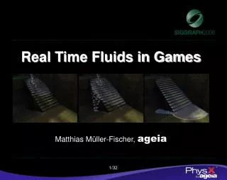
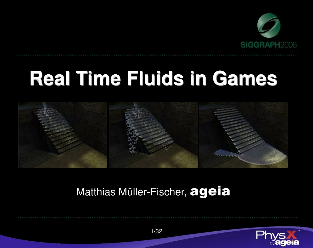
1. Real Time Fluids in Games Matthias Müller-Fischer, ageia 1/32

2. ageia • PhysX accelerator chip (PPU) • PhysX SDK (PPU accelerated) • rigid bodies + joints • cloth simulation • fluid simulation (SPH) 2/32

3. Real Time Fluids in Games • Fluids in Games • Heightfield Fluids • A very simple program • Mathematical background • Particle Based Fluids • Simple particle systems • Smoothed Particle Hydrodynamics (SPH) 3/32

4. Game Requirements • CHEAP TO COMPUTE! • 40-60 fps of which fluid only gets a small fraction • Low memory consumption • Must run on consoles • Stable even in non-realistic settings • Visually plausible 4/32

5. Solutions • Procedural Water • Unbounded surfaces, oceans • Heightfield Fluids • Ponds, lakes • Particle Systems • Splashing, spray, puddles 5/32

6. Procedural Animation • Simulate the effect, not the cause • No limits to creativity • E.g. superimpose sine waves:meshuggah.4fo.de, [2],[3] • See Splish Splash session! • Difficult but not impossible: • Fluid – scene interaction 6/32

7. Heightfield Fluids 7/32

8. u j i Heightfield Fluids u y x continuous discrete • Represent fluid surface as a 2D functionu(x,y) • Pro: Reduction from 3D to 2D • Cons: One value per (x,y) no breaking waves 8/32

9. Heightfield „Hello World“ • A trivial algorithm with impressive results! • Initialize u[i,j] with some interesting function, v[i,j]=0 loop v[i,j] +=(u[i-1,j] + u[i+1,j] + u[i,j-1] + u[i,j+1])/4 – u[i,j] v[i,j] *= 0.99 u[i,j] += v[i,j] endloop • Clamp on boundary e.g. def. u[-1,j] = u[0,j] 9/32

10. The Math Behind It Infinitesimal element u Vibrating string A f u fu x x x+dx • u(x) displacement normal to x-axis • Assuming small displacements and constant stress s • Force acting normal to cross section A is f =sA 10/32

11. Newton’s 2nd law for an infinitesimal segment (rAdx)utt = sAux|x+dx - sAux|x  r utt = s uxx PDE for the 1D String Infinitesimal element u Vibrating string A f u fu x x x+dx • Force acting normal to cross section A is f =sA • Component in u-direction fuuxsA (uxderivative w.r.t. x) 11/32

12. The 1D Wave Equation • For the string we have r utt = s uxx • Standard form: utt = c2 uxx, where c2= s/r • General solution:u(t) = a · f (x + ct) + b · f (x - ct) for any function f. • Thus, c is the speed at which waves travel 12/32

13. Intuition utt = c2uxx • Positive curvature is accelerated upwards • Negative curvature is accelerated downwards 13/32

14. The 2D Wave Equation • The wave equation generalizes to 2D as utt = c2(uxx + uyy) utt = c22u utt = c2u 14/32

15. vt+1[i,j]= vt[i,j] +tc2(u[i+1,j]+u[i-1,j]+u[i,j+1]+u[i,j-1]-4u[i,j])/h2 ut+1[i,j]= ut[i,j] +t vt+1[i,j] • We are where we started! (without damping) Discretization • Replace the 2nd order PDE by two first order PDEsut = vvt = c2 (uxx + uyy) • Discretize in space and time (semi-implicit Euler, time step t, grid spacing h) 15/32

16. Boundary conditions needed Mirror: Reflection Periodic: Wrap around Remarks on Heightfields • The simulation is only conditionally stable • Courant-Friedrichs-Lewy stability condition: cDt < h 16/32

17. Particle Based Fluids 17/32

18. With particle-particle interaction • Small puddles, blood, runnels • Small water accumulations Particle Based Fluids • Particle systems are simple and fast • Without particle-particle interaction • Spray, splashing 18/32

19. emitter • Generated by emitters,deleted when lifetime is exceeded Simple Particle Systems • Particles storemass, position, velocity, external forces, lifetimes mi xi • Integrated/dt xi = vid/dt vi = fi/mi vi fi 19/32

20. Particle-Particle Interaction • No interaction  decoupled system  fast • For n particles n2 potential interactions! • To reduce to linear complexity O(n)define interaction cutoff distance d d 20/32

21. d d Spatial Hashing • Fill particles into grid with spacing d • Only search potential neighbors in adjacent cells • Map cells [i,j,k] into 1D array via hash function h(i,j,k) 21/32

22. Repulsion Equilibrium Attraction Lennard-Jones Interaction • For simple fluid-like behavior: • k1, k2, m, n control parameters 22/32

23. Solving Navier-Stokes Eqn. • How formulate Navier-Stokes Eqn. on particles? • We need continuous fields, e.g. v(x) • Only have v1, v2, .. vnsampled on particles • Basic idea: • Particles induce smooth local fields • Global field is sum of local fields 23/32

24. Use scalar kernel function W(r) • Symmetric: W(|x-xi|) • Normalized:  W(x) dx = 1 r xi x SPH • Smoothed Particle Hydrodynamics • Invented for the simulation of stars [5] • Often used for real-time fluid simulation in CG [6] 24/32

25. Density of each particle • Mass conservation guaranteed Density Computation • Global density field 25/32

26. Gradient of smoothed attribute Smoothing Attributes • Smoothing of attribute A 26/32

27. Because particles follow the fluid we have: • The acceleration ai of particle i is, thus fi is body force evaluated at xi Equation of Motion 27/32

28. Symmetrize (SPH problem: actio  reactio) where pi = kri and k gas constant Pressure • The pressure term yields 28/32

29. Viscosity (simmetrized) Remaining Forces • Gravity as in simple particle systems 29/32

30. Remarks on SPH • Incompressibility • Pressure force reacts to density variation (bouncy) • Predict densities, solve for incompressibility [8] • Rendering • Marching cubes of density iso surface [6] • Sprites, depth buffer smoothing • Combine particles and heightfields [7] 30/32

31. References 1/2 [1] AGEIA: www.ageia.com, physx.ageia.com [2] A. Fournier and W. T. Reeves. A simple model of ocean waves, SIGGRAPH 86, pages 75–84 [3] D. Hinsinger, F. Neyret, M.P. Cani, Interactive Animation of Ocean Waves, In Proceedings of SCA 02 [4] A. Jeffrey, Applied Partial Differential Equations, Academic Press, ISBN 0-12-382252-1 31/32

32. References 2/2 [5] J. J. Monaghan, Smoothed particle hydrodynamics. Annual Review of Astronomy and Astrophysics, 30:543–574, 1992. [6] M. Müller, D. Charypar, M. Gross. Particle-Based Fluid Simulation for Interactive Applications, In Proceedings of SCA 03, pages 154-159. [7] J. O’Brien and J. Hodgins, Dynamic simulation of splashing fluids, In Computer Animation 95, pages 198–205 [8] S. Premoze et.al, Particle based simulation of fluids, Eurographics 03, pages 401-410 32/32