1 / 0

Prices

Prices. Lesson 11: Production. Readings and Assignments. The Young Economist 12-14. Teaser #10 :.

elon
Download Presentation

Prices

An Image/Link below is provided (as is) to download presentation Download Policy: Content on the Website is provided to you AS IS for your information and personal use and may not be sold / licensed / shared on other websites without getting consent from its author. Content is provided to you AS IS for your information and personal use only. Download presentation by click this link. While downloading, if for some reason you are not able to download a presentation, the publisher may have deleted the file from their server. During download, if you can't get a presentation, the file might be deleted by the publisher.

E N D

Presentation Transcript


  1. Prices

    Lesson 11: Production
  2. Readings and Assignments The Young Economist 12-14
  3. Teaser #10: A professor asked her research assistant to find out if the average wage for females rose or fell over a ten-year period.  That afternoon, the assistant returned and said, "I wasn't able to find anything on females, but I found out that the average wage for all workers fell during that period while the average wage for males rose.  It must be therefore be true that the average wage for females fell.""Not necessarily," sniffed the professor.  "It's possible that the average wage for females rose during that period, too."  How could that happen?
  4. Solution: As an example, suppose that 70% of the labor force was male and 30% was female and that their average wage rates were $10 and $7 respectively.  The average wage for all workers would be (70% X $10 + 30% X $7) = $9.10.  Now suppose that over the ten-year period the composition of the labor force changed so that 30% was male and 70% was female, and that their average wage rates rose to $11 and $8 respectively.  The average wage for all workers would fall to (30% X $11 + 70% X $8) = $8.90.
  5. Joke of the Day An economist and an accountant are walking along a large pond and see a frog jumping on the mud. The economist says:"If you eat the frog I'll give you $20,000!"The accountant checks his budget and figures out he's better off eating it, so he does and collects money.Continuing along they see another frog. The accountant says:"Now, if you eat this frog I'll give you $20,000."After evaluating the proposal the economist eats the frog and gets the money.
  6. Joke of the Day They go on. The accountant starts thinking: "Listen, we both have the same amount of money we had before, but we both ate frogs. I don't see us being better off."The economist says:
  7. Joke of the Day "Well, that's true, but you overlooked the fact that we've been just involved in $40,000 of trade."
  8. Economic Reasoning Principle # 3: People respond to incentives in predictable ways. Choices are influenced by incentives, the rewards that encourage and the punishments that discourage actions. When incentives change, behavior changes in predictable ways.
  9. $2 -$0.50 $1.50 π =
  10. I Don’t Know???
  11. $0.25 -$0.50 π = -$0.25
  12. P S Q
  13. P D Q
  14. Profits=Resource Groupies
  15. The Role of the Firm The firm is an economic institution that transforms factors of production into consumer goods – it: Organizes factors of production. Produces goods and services. Sells produced goods and services. Production is the name given to that transformation of factors into goods.
  16. The Role of the Firm A virtualfirm only organizes production. Virtual firms subcontract out all work. More and more of the organizational structure of business is being separated from the business. Not in the book but something to think about!
  17. The Structure of Production What is the ERE? ERE is a fictitious construct where the future is certain, a world where economic activities repeat themselves indefinitely. ERE is the final end state toward which the market would tend if all disturbing influences were held at bay. No uncertainty in the ERE ERE allows the conceptual distinction between profit and interest Because there is certainty, there can be no profits or losses in the ERE. However, there is still time preference, and hence interest.
  18. Remember the elements of Production? L=labor N=land (natural resources) K=capital Yet there are no true K goods, because they can all be traced to N and L All productive factors earn a (gross) rent or “hire price” per unit time in accordance with their marginal productivity, whether the factor is labor, a piece of land, or a machine.
  19. Land and Labor Born with Labor Homestead “raw” land Purchase thereafter Government’s job is to enforce these property definitions and rights.
  20. Capitalists Remember inputs, costs of production, have NO bearing on the price of a good Capitalists offer to pay workers (and land owners) immediately for services that will not yield finished consumer goods until the future. Capitalists are exchanging a present good (money) for a future good (the marginal product, in terms of the final consumer good, of the factor in question) The excess of the capitalists’ income from consumers, over the sum of payments they make to the owners of original factors, is due to interest (i.e., time preference), and not to any bargaining power or other “contribution” of the capitalists
  21. Specific vs. Nonspecific Factors Indispensable inputs to a productive process A set combination of specific and nonspecific factors A purely nonspecific factor would be one equally suited to the production of all possible products. It is clear that not all factors could be purely nonspecific, for in that case all factors would be purely interchangeable, i.e., there would be need for only one factor. L, the scarcest and most nonspecific factor
  22. The Production Function Pricing land, labor, capital Factors prices are based on costs of production and price of final goods. Derived Demand Production Function Max output with combination of inputs These tables are determined by engineers, but need to be understood by entrepreneurs. Law of Variable Proportions Ceteris paribus all but 1 within limits. In real world, probably in 100s if not 1000s.
  23. Factors of Production Law of Diminishing Marginal Returns Production Function (optimum combination) Complementary factors of production Specific Nonspecific Land, Labor, Capital Consumption Savings Roundabout production (more, but longer)
  24. Production Tables and Production Functions A production table shows the output resulting from various combinations of factors of production or inputs.
  25. Number of workers Marginal product Average product Total output 0 0 — 4 1 4 4 6 2 10 5 7 3 17 5.7 6 4 23 5.8 5 28 5.6 5 3 31 5.2 6 1 32 4.6 7 0 32 4.0 8 2 30 3.3 9 5 10 25 2.5 A Production Table
  26. Production Tables and Production Functions Marginal product is the additional output that will be forthcoming from an additional input, say a worker, other inputs remaining constant. Average product is calculated by dividing total output by the quantity of the input. Not in the text but an important concept to understand Average Cost later!
  27. Time and Stages of Production Immediate Everything made and ready for sale. Thus S is vertical in Immediate period Short-run Variable inputs and costs can be adjusted. Long-run All inputs and costs variable.
  28. The Production Function Law of Diminishing Returns: as more and more inputs are added to fixed quantities of other inputs, output increases, then slow, then declines. 3 Stages I: increasing II: diminishing III: declining This due to scarcity, otherwise if only stage I, why not grow all the world’s wheat on 1 acre!! This law is also called the flower pot law.
  29. Number of workers Total output Marginal product Average product 0 0 — 4 Increasing marginal returns 1 4 4 6 2 10 5 7 3 17 5.7 6 4 23 5.8 5 Diminishing marginal returns 28 5.6 5 3 31 5.2 6 1 32 4.6 7 0 32 4.0 8 2 Diminishing absolute returns 30 3.3 9 5 10 25 2.5 The Law of Diminishing Marginal Productivity
  30. The Law of Diminishing Marginal Productivity Diminishing absolute returns Diminishing marginal returns Diminishing marginal returns Diminishing absolute returns 32 7 30 28 6 26 24 TP 5 22 20 Increasing marginal returns 18 4 Output 16 Output per worker 14 3 12 10 2 8 AP 6 1 4 2 0 0 1 2 3 4 5 6 7 8 9 10 1 2 3 4 5 6 7 8 9 10 MP Number of workers Number of workers (a) Total product (b) Marginal and average product
  31. Relationships between TP, AP, MP, MR As TP goes up, MP is increasing, will reach max with 0 MP. Will decrease as MP is negative. As long as AP is rising, MP is increasing. When MP=AP MP is at max. As long as MP is higher than AP, AP rises.
  32. Relationships between TP, AP, MP, MR Never use inputs that are negative MP, never stop hiring in increasing MP (inefficient). A profit is made always in diminishing MP. (Stage II) If MR>MC (wage, rent) hire that factor.
  33. Productivity Total Product/# of inputs =AP Marginal Product (MP) Physical Capital Human Capital Technology Determines "wages"
  34. Cost of Production Accounting Cost Actual expenses plus depreciation (Explicit) Economic Cost Cost to a firm of using resources in production, plus Opportunity cost, the most valuable forgone alternative (Implicit) Sunk Cost Expenditure that has been made and cannot be recovered (Be Careful!)
  35. Cost of Production Example (Two building choices) A firm has two building choices. For Building 1, they have paid 500,000, and will pay 5,000,000 in the future For Building 2, they have not paid anything, and will pay 5,300,000 in the future. Although Building 2 is cheaper than Building 1, the firm will choose Building 1 because the 500,000 is sunk.
  36. Total Costs of Production Total Cost Total Cost =Variable Cost + Fixed Cost Fixed Cost. A cost that is actually incurred, but independent of the level of output Variable Cost. A cost that is actually incurred, and dependent of the level of output Example (Short Run). Capital K is fixed, and Labor L is variable; hence, the cost of K is a fixed cost, and the cost of L is a variable cost Total TC Fixed TFC Variable TVC
  37. More Costs+++ Average Costs AFC AVC ATC Marginal Costs (MC) Per unit cost
  38. L O M Total Cost Curves TC $400 VC 350 300 TC = VC + FC 250 Total cost 200 150 100 FC 50 0 2 4 6 8 10 20 30 Quantity of earrings
  39. ATC Area A Area C MC AVC Area B ATC AVC B A MC Q0 Q1 Relationship Between Marginal and Average Costs $90 80 70 60 50 40 Costs per unit 30 20 10 0 1 2 3 4 5 6 7 8 9 Quantity
  40. Profit MR=MC
  41. The U Shape of the Average and Marginal Cost Curves When output is increased in the short-run, it can only be done by increasing the variable input. The law of diminishing marginal productivity sets in as more and more of a variable input is added to a fixed input. The average total cost curve is the vertical summation of the average fixed cost curve and the average variable cost curve.
  42. Average and Marginal Cost Curves The average fixed cost curve slopes down continuously. It tells us that as output increases, the same fixed cost can be spread out over a wider range of output.
  43. Average and Marginal Cost Curves The marginal cost curve goes through the minimum point of the average total cost curve and average variable cost curve. Each of these curves is U-shaped.
  44. Productivity and Average and Marginal Cost Curves Marginal and average productivities fall and marginal costs rise. And when average productivity of the variable input falls, average variable cost rise. If the firm increased output enormously, the average variable cost curve and the average total cost curve would almost meet. The firm’s eye is focused on average total cost—it wants to keep it low.
  45. Relationship Between Marginal and Average Total Costs The marginal cost and average cost curves are related. When marginal cost exceeds average cost, average cost must be rising. When marginal cost is less than average cost, average cost must be falling. ATC = MC when ATC is at minimum
  46. Relationship Between Marginal and Average Variable Costs Marginal and average total cost reflect a general relationship that also holds for marginal cost and average variable cost. If MC > AVC, then AVC is rising. If MC = AVC, then AVC is at its low point. If MC < AVC, then AVC is falling.
  47. Relationship Between Marginal and Average Costs As long as average variable cost does not rise by more than average fixed cost falls, average total cost will fall when marginal cost is above average variable cost.
  48. The Perfectly Competitive Firm andIndustry in Short-Run Equilibrium
  49. To make their long-run decisions: Firms look at costs of various inputs and the technologies available for combining these inputs. Then decide which combination offers the lowest cost. The firm makes long-run decisions on the basis of the expected costs and expected usefulness of inputs. Making Long-Run Production Decisions
  50. Technical efficiency – as few inputs as possible are used to produce a given output. Technical efficiency is efficiency that does not consider cost of inputs. Technical Efficiency and Economic Efficiency
  51. Technical Efficiency and Economic Efficiency Economically efficient – the method that produces a given level of output at the lowest possible cost. It is the least-cost technically efficient process.
  52. Determinants of the Shape of the Long-Run Cost Curve The Law of Diminishing Marginal Productivity does not hold in the long run. All inputs are variable in the long run. The shape of the long-run cost curve is due to the existence of economies and diseconomies of scale.
  53. Economics of Scale Scale means size. Economies of scale: the decrease in per unit costs as the quantity of production increases and all resources are variable Diseconomies of scale: the increase in per unit costs as the quantity of production increases and all resources are variable Constant returns to scale: unit costs remain constant as the quantity of production is increased and all resources are variable
  54. Economies of Scale (MES) The minimum efficient level of production is the amount of production that spreads setup costs out sufficiently for firms to undertake production profitably.
  55. Economies of Scale (MES) The minimum efficient level of production is reached once the size of the market expands to a size large enough so that firms can take advantage of all economies of scale.
  56. Minimum Efficient Scale Most industries experience both economies and diseconomies of scale. The MES varies considerably across industries.
  57. Total Costs of Labor Total Cost of Machines Total Costs = TCL + TCM Average Total Costs = TC/Q Quantity 11 12 13 14 15 16 17 18 19 20 $381 390 402 420 450 480 510 549 600 666 $254 260 268 280 300 320 340 366 400 444 $635 650 670 700 750 800 850 915 1,000 1,110 $58 54 52 50 50 50 50 51 53 56 A Typical Long-Run Average Total Cost Table
  58. $64 62 60 Average total cost 58 56 Costs per unit Minimum efficient level of production 54 52 50 48 1 1 12 13 14 15 16 17 18 19 20 Quantity A Typical Long-Run Average Total Cost Curve
  59. Diseconomies of Scale Diminishing marginal productivity refers to the decline in productivity caused by increasing units of a variable input being added to a fixed input. Pay attention! Diminishing marginal productivity only applies in the Short-run!
  60. Diseconomies of Scale Diseconomies of scale occur on the right side of the long-run average cost curve where it is upward sloping, meaning that average cost is increasing.
  61. $64 62 60 Average total cost 58 56 Costs per unit 54 52 50 48 1 1 12 13 14 15 16 17 18 19 20 Quantity Economies and Diseconomies of Scale Economies of Scale Constant returns to Scale Diseconomies of Scale
  62. Importance of Economies and Diseconomies of Scale Economies and diseconomies of scale play important roles in real-world long-run production decisions. The long-run and the short-run average cost curves have the same U-shape, but the underlying causes of these shapes differ. Economies and diseconomies of scale account for the shape of the long-run total cost curve.
  63. What's wrong with this picture?
  64. Concept:  Economies of scale It's hard to imagine that Mark and Sally will make a profit with their business.  Suppose a customer asks them to deliver a small package to a city 200 miles away.  Unless they have many other packages going to the same city, they'd have to charge a lot just to cover their variable costs--labor, gas, and depreciation.   They wouldn't be able to compete against companies like UPS and FedEx, which can keep their costs down by handling a huge volume of parcels.
  65. WOW!!!!!!!!!!!!!
More Related