Download

1 / 24

E N D
Quicksort Quicksort is a well-known sorting algorithm developed by C. A. R. Hoare. The quick sort is an in-place, divide-and-conquer, massively recursive sort. It's essentially a faster in-place version of the merge sort. The quick sort algorithm is simple in theory, but very difficult to put into code (computer scientists tied themselves into knots for years trying to write a practical implementation of the algorithm, and it still has that effect on university students).
Quick Sort The recursive algorithm consists of four steps (which closely resemble the merge sort): • If there are one or less elements in the array to be sorted, return immediately. • Pick an element in the array to serve as a "pivot" point. (Usually the right-most element in the array is used.) • Split the array into two parts - one with elements larger than the pivot and the other with elements smaller than the pivot. • Recursively repeat the algorithm for both halves of the original array.
Quick Sort function quicksort(q) varlist less, pivotList, greater if length(q) ≤ 1return q select a pivot value pivot from q for each x in q except the pivot element if x < pivot then add x to less if x ≥ pivot then add x to greater add pivot to pivotList return concatenate(quicksort(less), pivotList, quicksort(greater))
85 24 63 45 17 31 96 50 Quick Sort – Visualization
85 24 63 45 17 31 96 50 Quick Sort – Visualization
85 24 63 45 17 31 96 50 50 24 45 17 31 Quick Sort – Visualization 85 63 96
85 24 63 45 17 31 96 50 50 24 45 17 31 Quick Sort – Visualization 85 63 96
85 24 63 45 17 31 96 50 50 24 45 17 31 24 17 85 63 Quick Sort – Visualization 85 63 96 31 45 96
85 24 63 45 17 31 96 50 50 24 45 17 31 24 17 85 63 Quick Sort – Visualization 85 63 96 31 45 96
85 24 63 45 17 31 96 50 50 24 45 17 31 24 17 85 63 Quick Sort – Visualization 85 63 96 31 45 96 17 24 63 85
85 24 63 45 17 31 96 50 50 24 45 17 31 17 24 63 85 Quick Sort – Visualization 85 63 96 31 45 96
85 24 63 45 17 31 96 50 50 17 24 31 45 Quick Sort – Visualization 63 85 96
17 24 31 45 50 63 85 96 Quick Sort – Visualization
85 24 63 45 17 31 96 50 85 63 96 50 24 45 17 31 31 45 96 17 24 63 85 24 17 85 63 Efficiency n = 8 Assuming the divide steps and the conquer steps take time proportional to n, then the runtime of each level is proportional to n. With logn + 1 levels, the runtime is O(nlogn).
Efficiency Best Case Situation Assuming that the list breaks into two equal halves, we have two lists of size N/2 to sort. In order for each half to be partitioned, (N/2)+(N/2) = N comparisons are made. Also assuming that each of these list breaks into two equal sized sublists, we can assume that there will be at the most log(N) splits. This will result in a best time estimate of O(N*log(N)) for Quicksort.
Efficiency Worst Case Situation In the worst case the list does not divide equally and is larger on one side than the other. In this case the splitting may go on N-1 times. This gives a worst-case time estimate of O(N²). Average Time The average time for Quicksort is estimated to be O(N*log(N)) comparisons.
Efficiency The disadvantage of the simple version previously stated is that it requires extra storage space. The additional memory allocations required can also drastically impact speed and cache performance in practical implementations. There is a more complicated version which uses an in-place partition algorithm.
In-Place Quick Sort • Sorting in place • “Instead of transferring elements out of a sequence and then back in, we just re-arrange them.” • Uses a constant amount of memory • Efficient space usage • Algorithm inPlaceQuickSort • Runs efficiently when the sequence is implemented with an array
85 24 63 45 17 31 96 50 In-Place Quick Sort Visualization
85 85 31 24 24 24 63 63 63 45 45 45 17 17 17 85 31 31 96 96 96 50 50 50 l++ while its value <= p AND l <= r r-- while its value >= p AND r >= l l r p swap l and r (as long as l < r) l r p In-Place Quick Sort Visualization Pivot p = element at the right bound index l = leftBound index r = rightBound – 1 l r p while l <= r
31 85 31 31 85 24 24 24 24 24 63 63 63 63 17 45 45 45 45 45 17 17 17 63 17 31 85 85 85 31 96 96 96 96 96 50 50 50 50 50 l++ while its value <= p AND l <= r r-- while its value >= p AND r >= l l r p swap l and r (as long as l < r) l r p In-Place Quick Sort Visualization Pivot p = element at the right bound index l = leftBound index r = rightBound – 1 l r p while l <= r l r p l r p
31 85 31 31 85 31 31 24 24 24 24 24 24 24 17 63 17 63 63 17 63 45 45 45 45 45 45 45 17 63 17 17 50 17 63 85 31 85 85 31 85 85 96 96 96 96 96 96 96 50 63 50 50 50 50 50 In-Place Quick Sort Visualization Pivot p = element at the right bound index l = leftBound index r = rightBound – 1 l r p while l <= r l++ while its value <= p AND l <= r r-- while its value >= p AND r >= l l r p swap l and r (as long as l < r) l r p l++ while its value <= p AND l <= r r-- while its value >= p AND r >= l l r p whenl > r swap l and p l r p sort(left = leftBound, right = l – 1) sort(left = l + 1, right = rightBound) r l p r l p
Randomized Quick Sort • Variation of the quick sort algorithm • Instead of selecting the last element as the pivot, select an element at random • Expected runtime efficiency will always be O(nlogn)