Download
1 / 38
380 likes | 471 Views
PH D THES IS DEFENSE , 2004 – 2007 NICOLAS RASCLE. IMPACT OF WAVES ON THE OCEAN CIRCULATION. Thesis supervisor : Fabrice ARDHUIN (SHOM, Brest) Financ ial support : DGA / CNRS Laborato ries :

E N D
PHD THESIS DEFENSE, 2004 – 2007 NICOLAS RASCLE IMPACT OF WAVESON THE OCEAN CIRCULATION Thesis supervisor :FabriceARDHUIN (SHOM, Brest) Financial support : DGA/ CNRS Laboratories : (1) Centre Militaire d’Océanographie, Service Hydrogaphique et Océanographique de la Marine, Brest (2) Laboratoire de Physique des Océans, Université de Bretagne Occidentale, Brest
PHD THESIS DEFENSE, 2004 – 2007 NICOLAS RASCLE Introduction General concepts Impact of waves on the currents of the surface layer in the open ocean (1D) Impact of waves on the coastal and nearshore currents (3D) Conclusion 2 / 38
INTRODUCTION Contextof the thesis : interactions Atmosphere / Waves / Ocean Subject of the thesis : impact of waves on the ocean circulation Atmosphere Energy and momentum exchanges Waves Ocean 3 / 38
INTRODUCTION • The waves : • Impact on ocean surface drift ? • Impact on the mixing of the near-surface ocean ? • Impact on the ocean circulation at global scale ? • Impact on the currents close to the coast ? 4 / 38
INTRODUCTION • Try to bring a better knowledge of: • surface currents • near-shore and inner-shelf currents • temperature and other tracers close to the surface • Practical applications ? • survey of surface drifts of particles or objects • (pollutions, search and rescue) • survey of drifting materials in nearshore and costal waters • (larvae recrutement, sedimentary transport) • vertical mixing in the near-surface ocean • (formation of diurnal thermoclines, blooms) • teledetection • (velocities and slopes of the surface) • Analyse of the existing ocean circulation models(without waves) • Importance of waves ? 5 / 38
GENERAL Waves ? z x Short gravity wave : Wavelength = 100 m Period = 10 s Height = 1 m But the mean length scales for the variations of the wave field are longer : 100 km, a few days… 6 / 38
GENERAL Eulerian description of the Stokes drift Waves (linear) = acos(kx-t) u = acos(kx-t) exp(kz) si z < w = asin(kx-t) exp (kz) z z u x The Stokes transport occurs between crests and throughs. 7 / 38
GENERAL Lagrangienne description of the Stokes drift Waves = acos(kx-t) u = acos(kx-t) exp(kz) si z < w = asin(kx-t) exp (kz) z z u =Us x The orbits of particles are not closed : -> Stokes drift The transport occurs over a depth of the order of a ten of meters. 8 / 38
GENERAL 2 difficulties to model the current when waves are present : • The motion of the free surface -> imposes a special averaging close to the surface 2. Different physics between the Stokes drift and the mean current (vertical mixing, propagation : Cg >> u, …) -> imposes to separate waves and mean current Use of the Generalized Lagrangian Mean theory (GLM) (Andrews et McIntyre, 1978, Ardhuin et al., 2007) 9 / 38
GENERAL Once made aGLM averaging,one obtains : • The free surface is moved back to its mean position. • The Stokesdrift in agreement with its Lagrangian description. • The mean currentdescribed by aquasi-Eulerianmean, and not an Eulerian mean. • Lagrangian drift = quasi-Eulerian velocity + Stokes drift : • Wave field dynamics<-/-> Quasi-Eulerian current dynamics 10 / 38
GENERAL Dynamics of the mean current dynamics of the total Lagrangian drift Ex : Equilibrium in an horizontaly uniform case(and without stratification) Coriolis Turbulent diffusion Stokes-Coriolis force : (action of the Coriolis force on the wave field, momentum then given to the mean flow) Wind stress 11 / 38
GENERAL The Stokes-Coriolis force (Hasselmann, 1970) Case of a wind sea Wind waves At long time scales, the Stokes-Coriolis force creates a (vertically integrated) transport which compensatesthe Stokes transport -> no modificationsof the Ekman pumping by waves (Hasselmann, 1970) -> no modificationsof the ocean circulation at global scale Stokes transport Wind stress Stokes-Coriolis transport Ekman transport y Stokes-Coriolis force x 12 / 38
GENERAL Stokes-Coriolis force (Hasselmann, 1970) • Vertically integrated, no net transport induced by waves. • But there still might be a net Lagrangian drift : Transport of Stokes-Coriolis Stokes transport Mean Current Lagrangian drift Stokes drift + vertical mixing No net Lagrangian drift Case of a wind sea Case of a long swell 13 / 38
PART 1 : VELOCITIES IN THE SURFACE LAYER Partie 1 : Impact of waves on the surface currents (1D) Surface drift offshore : • Surface drift due to the wind : 2 or 3% of U10(Huang, 1979) • The Ekman currents at the surface strongly depend on thevertical mixing Kz : 0.5 to 4% of U10 • Stokes drift of waves of same magnitude order : 3% de U10(Kenyon, 1969) Coherent description? Which one dominates the surface drift ? 14 / 38
PART 1 : VELOCITIES IN THE SURFACE LAYER The Stokes drift Modelisationof the wave field by a freq-dir spectrum (Kudryavtsev et al., 1999) of the sea surface elevation (spectral approach in phase in the mean) : Stokes drift (uncorrelated phases) : 15 / 38
PART 1 : VELOCITIES IN THE SURFACE LAYER Spectra f^3 E(f) (Stokes drift at the surface) Energie spectra E(f) (=height^2) Height, Periods Hs=1.6m, Tp=5.5s Hs=2.8m, Tp=8s Hs=2.8m, Tp=8s Hs=2.8m, Tp=12s Stokes drifts Us=10. cm/s Us=12. cm/s Us=5.2 cm/s Us=1.6 cm/s (Wind : U10=10 m/s) Young wind sea Developed wind sea Short swell Long swell --- 16 / 38
PART 1 : VELOCITIES IN THE SURFACE LAYER The Stokes drift • For a fully-developed wind sea : • at the surface 1.2% of U10 (< Kenyon, 1969) • up to 30% of the Ekman transport(< McWilliams et Restrepo, 1999) • affect depths of • 10-40m • For the swell, small surface Stokes drift. (Wind : U10=10 m/s) Young wind sea Developed wind sea Short swell Long swell --- 17 / 38
Roughness length TKE surface flux PART 1 : VELOCITIES IN THE SURFACE LAYER Vertical mixing : effect of waves 1D TKE model (Craig et Banner, 1994) Mixing length : prescribed TKE calculation diffusion production dissipation Injection of TKE by the dissipation of the wave field : 18 / 38
EQUATIONS POUR LE COURANT QUASI-EULERIEN PART 1 : VELOCITIES IN THE SURFACE LAYER Vertical mixing : effect of waves • Dominant parameter : the roughness length A dimensional analysis, confirmedby mesurements of dissipation of TKE :(Terray et al., 1996) • -> The surface mixing increases with the wave growth. Proxy for the scale of the breaking waves 19 / 38
EQUATIONS POUR LE COURANT QUASI-EULERIEN PART 1 : VELOCITIES IN THE SURFACE LAYER Consequence for the Lagrangian drift : • The drift at the surface essentiallycomes from the Stokes drift when the waves are developed.(Rascle et al., 2006) (Vent : U10=10 m/s) Lagrangian drift Stokes drift Mean current 20 / 38
PART 1 : VELOCITIES IN THE SURFACE LAYER Validations : The observations of TKE dissipation The observations of Lagrangian drifts The observations of quasi-Eulerian currents • TKE model built from observations of TKE dissipation • z0 tuned in consequence • Still some uncertainties(Gemmrich et Farmer, 1999, 2004) 21 / 38
PART 1 : VELOCITIES IN THE SURFACE LAYER Validations : The observations of TKE dissipation The observations of Lagrangian drifts The observations of quasi-Eulerian currents • Few available(complete) data • Estimation to 2-3% of U10 at the surface (Huang, 1979) • Note the current work of Kudryavtsev et al. on the vertical shears • of drifters observations (Kudryavtsev et al., 2007, submitted) 22 / 38
PART 1 : VELOCITIES IN THE SURFACE LAYER Validations : The observations of TKE dissipation The observations of Lagrangian drifts The observations of quasi-Eulerian currents 2 datasets examined : LOTUS 3(1982, Sargassian sea) (Price et al., 1987, Polton et al. 2005) SMILE(1989, californian shelf) (Santala, 1991) VMCM Short field experiment (2 days) Wave follower Mesurement very close to the surface Bias corrections Long field experiment (160 days) Classical mooring Minimum depth of measurements : 5m 23 / 38
PART 1 : VELOCITIES IN THE SURFACE LAYER Validations : 3.the observations ofquasi-Eulerian currents Vertical shears close to the surface (SMILE) 1D TKE model with stratification (Noh, 1996, Gaspar et al. 1990) • Small downwind shear -> validates the wave-induced near-surface mixing • Crosswind shear ? • No evidence of the Stokes-Coriolis effect on the crosswind component 24 / 38
PART 1 : VELOCITIES IN THE SURFACE LAYER Validations : 3.the observations ofquasi-Eulerian currents • Complete spirales(LOTUS 3) • Very good agreement model / data. • No evidence of the wave-induced mixing (at 5m deep and more) • No evidence of the Stokes-Coriolis transport (contrary to Polton et al., 2005 without stratification). Probably because of a wave-induced bias. 1D TKE model with stratification nudging.(Noh, 1996, Gaspar et al. 1990) 25 / 38
PART 1 : VELOCITIES IN THE SURFACE LAYER Summary - Conclusion • Impact of waves on the currents of the surface layer in the open ocean (1D) • Problematic of surface drift offshore (1D) • re-evaluation of the Stokes drift • evaluation of the mean current by parameterizing the wave-induced mixing • evaluation of the Lagrangian drift at the surface • -> the Stokes drift dominates (Rascle et al., 2006) • comparison with mean currents observations • -> carefull conclusions (Stokes-Coriolis ?) (Rascle et Ardhuin, 2007, soumis) 26 / 38
PART 2 : INNER-SHELF AND SURF ZONE CURRENTS Part 2 : Impact of waves on the coastal and nearshore currents (3D) Coastal zone Inner-shelf zone Surf zone Waves Breaking Shoaling Tide Wind Coriolis Stratification -10m Tide Waves -50m Transition ? Poorly understood dynamics Importance of radiation stress ? of (Stokes-) Coriolis ? Important zone Radiation stresses 2D Bousinessq models Primitive equation models • 2 goals : • understand the inner-shelf dynamics • model : develop a 3D model (primitives equations) to resolve from the offshore to the surf zone 27 / 38
PART 2 : INNER-SHELF AND SURF ZONE CURRENTS For the hydrodynamics of that inner-shelf zone, one needs complete equations (3D) of the forcing of currents by waves : • Mellor 2003 -> problem in the vertical profile of the radiation stress • (Ardhuin et al., 2007 b) • McWilliams et al., 2004 -> adiabatic • Ardhuin, Rascle et Belibassakis 2007 (GLM) • Momentum: • Mass: • Tracers: 28 / 38
PART 2 : INNER-SHELF AND SURF ZONE CURRENTS My work : Implement those equations in ROMS to solve the mean circulation forced by waves : extension of a coastal model to the surf zone 2. Tests on an academic case 3. Description of the dynamics with GLM formalism, Comparison to existing descriptions of the surf-zone and inner-shelf zone 29 / 38
PART 2 : INNER-SHELF AND SURF ZONE CURRENTS 1. Academic case Straight and infinite coast Waves Breaking Set-down Set-up Jet Calculation of waves, of Stokes drift Model of Thornton and Guza Forcing Calculation of the mean current ROMS model, modified primitive equations (GLM equations) dt = 3 s Kz = 0.03 m2/s 40 vertical levels f = 10-4 s-1 4 km 400 points (dx=10 m) 30 / 38
Mom. : • Mass: • Tracers: PART 2 : INNER-SHELF AND SURF ZONE CURRENTS 2. Implementation in ROMS : • Primitives equations model • Sigma coordinates • Just solves the mean current : Stokes drift comes from the wave model • Baroclinic / barotropic time stepping -> complicates the modification of the equations (tracer) 31 / 38
PART 2 : INNER-SHELF AND SURF ZONE CURRENTS • Momentum : • horizontal and vertical vortex forces(McWilliams et al., 2004) 3. Description of the dynamics in the GLM theory Littoral jet Horiz. vortex force : shifts the jet towards the beach Vertical vortex force : slow down the jet Vorticity ω3 < 0 Vorticity ω3 > 0 32 / 38
PART 2 : INNER-SHELF AND SURF ZONE CURRENTS 3. Description of the dynamics in the GLM theory • Momentum : • Stokes-Coriolis force Stokes transport Transport of the mean current Stokes-Coriolis force -> transition towards the off-shore dynamics (Lentz et al., 2007, submitted) Inner-shelf zone Surf zone 33 / 38
PART 2 : INNER-SHELF AND SURF ZONE CURRENTS 3. Description of the dynamics in the GLM theory • tracers : • What about the Lagrangian drift ? • Non-linear effectson the Stokes drift in shallow water • The Stokes is important compared to the cross-shore currents (Monismith et Fong, 2004) • And even more if the waves are non-linear. • Can lead to an important Lagrangian drift towards the beach at the surface,even outside the surf zone 34 / 38
PART 2 : INNER-SHELF AND SURF ZONE CURRENTS Summary - Conclusion Impact of waves on the coastal and nearshore currents (3D) Goal : link between shelf and surf-zone, through the inner-shelf zone • Equations (recently developed) for the 3D interactions between waves and current (Ardhuin et al., 2007) • Implementation in a coastal model (ROMS) • Academic test • What new on the dynamics with the GLM theory ? horizontal and vertical vortex forces (effects partly discussed by Newberg et Allen, 2007) Stokes-Coriolis effect for the transition towards the offshore dynamics (observed by Lentz et al., 2007, submitted) analyse of the Lagrangian drift (non-linear effects on the Stokes drift in shallow water) 35 / 38
GENERAL CONCLUSION • The waves : • Impact on the ocean circulation at global scale ? • Impact on ocean surface drift ? • Impact on the mixing of the near-surface ocean ? • Impact on the currents close to the coast ? • Use of a set of equations which separates waves and currents • (GLM) (Ardhuin et al., 2007) • What do my work bring to answer to those (3 last) questions ? 36 / 38
GENERAL CONCLUSION • The surface drift offshore : • dominated by the waves Stokes drift • the mean current is weaker at the surface • but note that the surface drift of a swell is small (-> the drift still depends on the wind) • The near-surface mixing : • depends on the waves developement • strong when the waves are developed -> impact on the mixed layer, on the vertical distributions of drifting materials (impact on the Random Walk ?) • one needs waves to get simultaneously realistic (strong) surface mixing and realistic surface drift • The coastal currents : • strong current induced by waves in the surf zone (that’s not new !) • but also a few things new on the dynamics of the surf zone and of the inner-shelf zone • there can be strong cross-shore drifts induced by waves, even in the inner shelf zone 37 / 38
FUTURE WORKS Following the present work : • Mixing model :Validations of the roughness length with TKE dissipation measurements (Gemmrich and Farmer, 2004)Re-evaluation of the TKE flux at the surface (Phd thesis of J. F. Fillipot) • Model of the offshore surface drift : Validations with the observations ofLagrangian drifts(Kudryavtsev et al., 2007, soumis) • Inner-shelf model : Comparison of the model with the mesurements of Lentz et al., 2007, submitted Possible future works : • Parameterizations of the Stokes drift and of the radiation stress for non-linear realistic waves • Studies of rip-current and other 3D problems involving the coupling of waves and currents. Impact of the horizontal and vertical vortex force. • Applications to material drifts in coastal and off-shore waters. • … Thank you. 38 / 38