Download
1 / 56
560 likes | 785 Views
ROMS 4D-Var: The Complete Story. Andy Moore Ocean Sciences Department University of California Santa Cruz & Hernan Arango IMCS, Rutgers University. Acknowledgements. ONR NSF. Chris Edwards, UCSC Jerome Fiechter, UCSC Gregoire Broquet, UCSC Milena Veneziani, UCSC

E N D
ROMS 4D-Var: The Complete Story Andy Moore Ocean Sciences Department University of California Santa Cruz & Hernan Arango IMCS, Rutgers University
Acknowledgements • ONR • NSF • Chris Edwards, UCSC • Jerome Fiechter, UCSC • Gregoire Broquet, UCSC • Milena Veneziani, UCSC • Javier Zavala, Rutgers • Gordon Zhang, Rutgers • Julia Levin, Rutgers • John Wilkin, Rutgers • Brian Powell, U Hawaii • Bruce Cornuelle, Scripps • Art Miller, Scripps • Emanuele Di Lorenzo, Georgia Tech • Anthony Weaver, CERFACS • Mike Fisher, ECMWF
Outline • What is data assimilation? • Review 4-dimensional variational methods • Illustrative examples for California Current
Best Linear Unbiased Estimate (BLUE) Prior hypothesis: random, unbiased, uncorrelated errors Error std: Find: A linear, minimum variance, unbiased estimate is minimised so that
Best Linear Unbiased Estimate (BLUE) Let OR Posterior error:
Data Assimilation fb(t), Bf ROMS bb(t), Bb xb(0), B Obs, y xb(t) x(t) time Model solutions depends on xb(0), fb(t), bb(t), h(t)
Data Assimilation Find initial condition increment corrections for model error boundary condition increment forcing increment that minimizes the variance given by: Tangent Linear Model Obs Error Cov. Innovation Background error covariance
OR 4D-Variational Data Assimilation (4D-Var) At the minimum of J we have : Obs, y xb(t) x(t) xa(t) time
Matrix-less Operations There are no matrix multiplications! Zonal shear flow
Matrix-less Operations There are no matrix multiplications! Adjoint ROMS Zonal shear flow
Matrix-less Operations There are no matrix multiplications! Adjoint ROMS Zonal shear flow
Matrix-less Operations There are no matrix multiplications! Covariance Zonal shear flow
Matrix-less Operations There are no matrix multiplications! Covariance Zonal shear flow
Matrix-less Operations There are no matrix multiplications! Tangent Linear ROMS Zonal shear flow
Matrix-less Operations There are no matrix multiplications! Tangent Linear ROMS Zonal shear flow
Representers = A representer Green’s Function A covariance Zonal shear flow
Solve linear system of equations! A Tale of Two Spaces K = Kalman Gain Matrix
Solve linear system of equations! A Tale of Two Spaces
A Tale of Two Spaces Model space searches: Incremental 4D-Var (I4D-Var) Observation space searches: Physical-space Statistical Analysis System (4D-PSAS)
An alternative approach in observation space: The Method of Representers vector of representer coefficients matrix of representers (Bennett, 2002) : solution of finite-amplitude linearization of ROMS (RPROMS) R4D-Var
Representers = A representer Green’s Function A covariance Zonal shear flow
4D-Var: Two Flavours Strong constraint: Model is error free Weak constraint: Model has errors Only practical in observation space
4D-Var Summary Model space: I4D-Var, strong only (IS4D-Var) Observation space: 4D-PSAS, R4D-Var strong or weak
Former Secretary of Defense Donald Rumsfeld
Why 3 4D-Var Systems? • I4D-Var: traditional NWP, • lots of experience, • strong only (will phase out). • R4D-Var: formally most correct, • mathematically rigorous, • problems with high Ro. • 4D-PSAS: an excellent compromise, • more robust for high Ro, • formally suboptimal.
The California Current System (CCS) 10km grid 30km grid Veneziani et al (2009) Broquet et al (2009)
The California Current System (CCS) June mean SST (2000-2004) 10km grid 30km grid COAMPS 10km winds; ECCO open boundary conditions fb(t) bb(t) Veneziani et al (2009); Broquet et al (2009)
3km grid Chris Edwards
Observations (y) CalCOFI & GLOBEC SST & SSH Ingleby and Huddleston (2007) TOPP Elephant Seals ARGO
Solve linear system of equations! A Tale of Two Spaces
CCS 4D-Var From previous cycle ECCO COAMPS
Model Space vs Observation Space (I4D-Var vs 4D-PSAS vs R4D-Var) Model space (~105): Observation space (~104): J J Both matrices are conditioned the same with respect to inversion (Courtier, 1997) Jmin # iterations # iterations (1 outer, 50 inner, Lh=50 km, Lv=30m) July 2000: 4 day assimilation window STRONG CONSTRAINT
SST Incrementsdx(0) Inner-loop 50 I4D-Var 4D-PSAS R4D-Var Model Space Observation Space Observation Space
Initial conditions vs surface forcing vs boundary conditions J No assimilation i.c. only i.c. + f i.c.+ f + b.c. IS4D-Var, 1 outer, 50 inner 4 day window, July 2000
Model Skill RMS error in temperature No assim. Assim. 14d frcst I4D-Var (1 outer, 20 inner, 14d cycles Lh=50 km, Lv=30m) Broquet et al (2009)
Surface Flux Corrections, (I4D-Var) Wind stress increments (Spring, 2000-2004) Heat flux increments (Spring, 2000-2004) Broquet
Model Error h(t) Model error prior std in SST
Solve linear system of equations! A Tale of Two Spaces
Model Space vs Observation Space (I4D-Var vs 4D-PSAS vs R4D-Var) Model space (~108): Observation space (~104): J J Jmin # iterations # iterations (1 outer, 50 inner, Lh=50 km, Lv=30m) July 2000: 4 day assimilation window STRONG vs WEAK CONSTRAINT
4D-Var Post-Processing • Observation sensitivity • Representer functions • Posterior errors
Assimilation impacts on CC No assim Time mean alongshore flow across 37N, 2000-2004 (30km) IS4D-Var (Broquet et al, 2009)
Observation Sensitivity What is the sensitivity of the transport I to variations in the observations? What is ?
Observations (y) CalCOFI & GLOBEC SST & SSH Ingleby and Huddleston (2007) TOPP Elephant Seals ARGO
Observation Sensitivity SSH day 4 SST day 4 Sverdrups per metre Sverdrups per degree C Sensitivity of upper-ocean alongshore transport across 37N, 0-500m, on day 7 to SST & SSH observations on day 4(July 2000) Applications: predictability, quality control, array design
CalCOFI GLOBEC depth Sv/deg C Sv/psu Sv/deg C Sv/psu Applications: predictability, quality control, array design