Download
1 / 58
590 likes | 609 Views
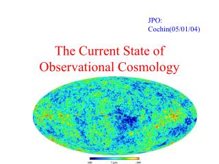
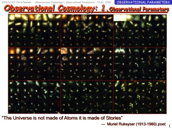
Observational Cosmology: 3. Structure Formation. “ An ocean traveler has even more vividly the impression that the ocean is made of waves than that it is made of water. ”. Arthur S. Eddington (1882-1944). 3.1: Isotropy & Homogeneity on the Largest Scales.

E N D
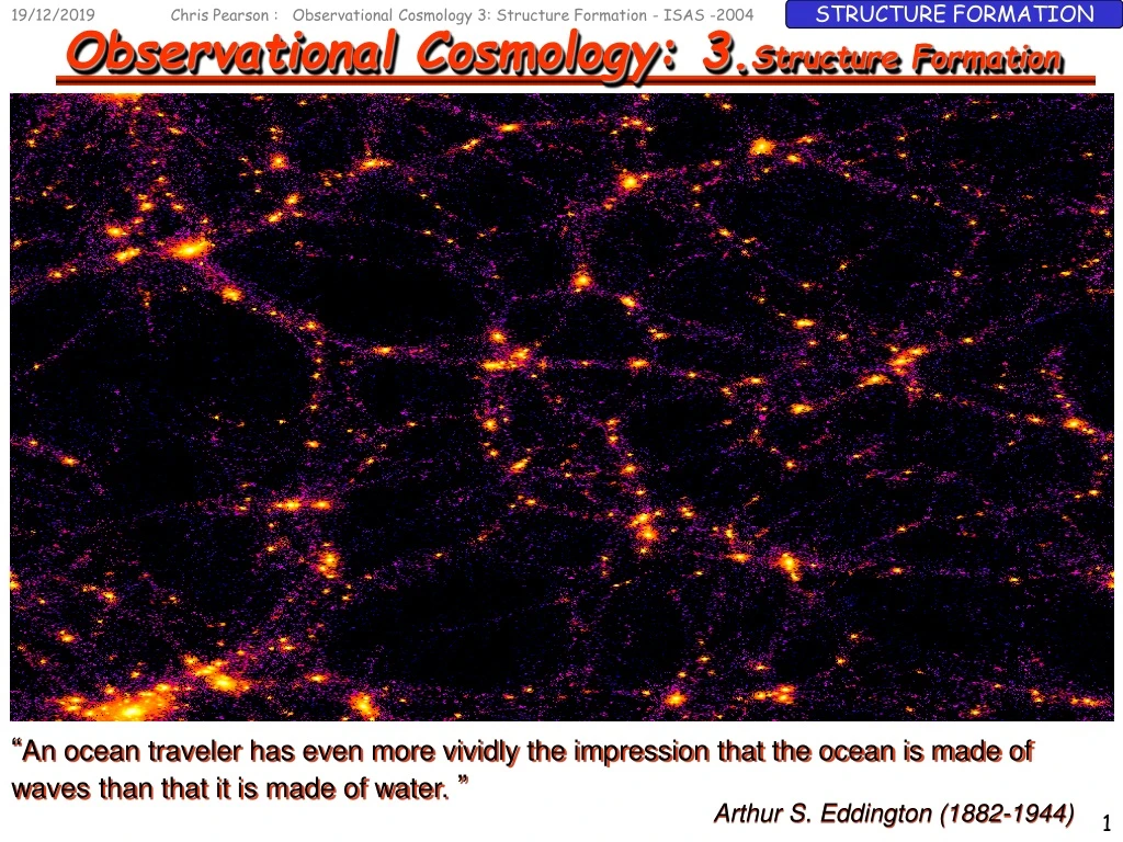
Chris Pearson : Observational Cosmology 3: Structure Formation - ISAS -2004 Observational Cosmology: 3.Structure Formation “An ocean traveler has even more vividly the impression that the ocean is made of waves than that it is made of water. ” Arthur S. Eddington (1882-1944)
Chris Pearson : Observational Cosmology 3: Structure Formation - ISAS -2004 3.1: Isotropy & Homogeneity on the Largest Scales Isotropy and Homogeneity on the largest scales Cosmological Principle: The Universe is Homogeneous and Isotropic True on the largest Scales Radiation: CMB - Isotropic to 1 part in 105, 0.003%, 2mK Matter: Large scales > 100Mpc (Clusters / Superclusters) : Universe is smooth Radio Sources: isotropic to a few percent Small scales : Highly anisotropic
Chris Pearson : Observational Cosmology 3: Structure Formation - ISAS -2004 ~1000Mpc • Walls • Filaments • Clusters • Superclusters • Voids 3.1: Isotropy & Homogeneity on the Largest Scales Isotropy and Homogeneity on the largest scales 200Mpc
Chris Pearson : Observational Cosmology 3: Structure Formation - ISAS -2004 Density perturbation • 1) Primordial Quantum Fluctuations • Gaussian Fluctuations from inflation • 2) Cosmic Defects • Defects from phase transitions • Cosmic String • Domain Walls • Textures • Scale Free Harrison - Zeldovich spectrum model: • Fluctuations have the same amplitude when they enter the horizon ~ d ~ 10-4 • Scale free Harrison-Zeldovich Spectrum of power 3.2: The Growth of Structure Origin of LSS today - primordial density fluctuations Primordial Density Fluctuations
Chris Pearson : Observational Cosmology 3: Structure Formation - ISAS -2004 3.2: The Growth of Structure Primordial Density Fluctuations
Chris Pearson : Observational Cosmology 3: Structure Formation - ISAS -2004 r ISOTHERMAL FLUCTUATIONS Fluctuations in matter ONLY No perturbations in the Temperature r ADIABATIC FLUCTUATIONS Fluctuations in matter and radiation (changes in volume in the early Universe change in number densities) r ISO-CURVATURE / ISENTROPIC FLUCTUATIONS No Perturbations in the density field Fluctuations in the matter relative to the radiation dm-dg 3.2: The Growth of Structure Primordial Density Fluctuations Fluctuations in radiation field leave scar on CMB observed as deviations from 2.73K BB
Chris Pearson : Observational Cosmology 3: Structure Formation - ISAS -2004 Consider a homogeneous universe of average density Embed a sphere of mass, with over density Sphere collapses from rest equilibrium under self gravity During Collapse r = r(1+d) r r M Solutions of the form = Where, is the dynamical free fall time 1 2 1 2 Only exponentially increasing term survives 3.2: The Growth of Structure The Jeans Length Conclusion: Density perturbations will grow exponential under the influence of self gravity
Chris Pearson : Observational Cosmology 3: Structure Formation - ISAS -2004 = the sound speed Equation of State for an Ideal Gas ( fundamental cosmology 5.3) GRAVITY Compression Pressure Acoustic Oscillations Pressure Gradient - Resists Collapse if a pressure gradient can be created over a timescale given by tJ < tff Pressure Expansion JEANS LENGTH JEANS MASS 3.2: The Growth of Structure The Jeans Length In absence of pressure, an overdense region collapses on order of the free fall time Define a critical length over which density perturbation will be stable against collapse under self gravity
Chris Pearson : Observational Cosmology 3: Structure Formation - ISAS -2004 3.2: The Growth of Structure Formal Jeans Theory Continuity Equation Euler Equation Poisson Equation Entropy Equation
Chris Pearson : Observational Cosmology 3: Structure Formation - ISAS -2004 Friedmann eqn. (k=0) expansion rate of Universe given by Hubble parameter Free Fall Time Jeans Length Photon sound speed (w=1/3) At decoupling (z=1089) Super-horizon scales Sub horizon scales cannot grow 3.2: The Growth of Structure Jeans Mass, Silk Mass and the decoupling epoch Before epoch of decoupling, photons and Baryons bound together as a single fluid This mass is larger than the largest Supercluster today !
Chris Pearson : Observational Cosmology 3: Structure Formation - ISAS -2004 Photon sound speed Baryon sound speed After decoupling Jean’s Length Jean’s Mass after decoupling 3.2: The Growth of Structure Jeans Mass, Silk Mass and the decoupling epoch After epoch of decoupling, photons and Baryons behave as separate fluids This mass is approximately the same mass as Globular Cluster today ! Until decoupling, structures over scales of globular clusters up to superclusters could not grow
Chris Pearson : Observational Cosmology 3: Structure Formation - ISAS -2004 Asymptotic value 18 unstable 16 14 12 lg(MJ) {Mo} unstable 10 Acoustic oscillation 8 recombination Matter-radiation equality 6 4 Radiation dominated Matter dominated 2 9 7 5 3 2 lg(Tr) {K} THE SILK MASS 3.2: The Growth of Structure Jeans Mass, Silk Mass and the decoupling epoch • Close to decoupling / recombination : Baryon/photon fluid coupling becomes inefficient • Photon mean free path increases diffuse / leak out from over dense regions • Photons / baryons coupled smooth out baryon fluctuations • Damp fluctuations below mass scale corresponding to distance traveled in one expansion timescale
Chris Pearson : Observational Cosmology 3: Structure Formation - ISAS -2004 Free Fall Time Hubble Expansion Expanding Universe r Embed a sphere of density r, in a homogeneous universe r M Total Gravitational acceleration at surface of the sphere r = r(1+d) During Collapse/expansion For homogeneous, isotropic universe,d=0 = 2 1 Subtracting the homogeneous component For a static universe, H=0 1 2 Extra term in expanding universe HUBBLE FRICTION slows the growth of the density pertubations 3.2: The Growth of Structure Growth of Perturbations in an expanding universe : The Hubble Friction Growth of structure - competition between 2 factors:
Chris Pearson : Observational Cosmology 3: Structure Formation - ISAS -2004 Solution: Radiation Era Wm<<1 Fluctuations in matter (non-baryonic) can only grow logarithmically Lambda Era H=HL= Const Solution: F;uctuations in matter tend to a constant fractional amplitude. Solution: Matter Era (Wm=1, H=2/3t) Growing mode and a decaying mode exist Density fluctuations in a flat, matter dominated Universe grow as 3.2: The Growth of Structure Growth of Perturbations in an expanding universe Rewrite in terms of density parameter
Chris Pearson : Observational Cosmology 3: Structure Formation - ISAS -2004 DARK MATTER Dark Matter Condenses at earlier time Matter then falls into DM gravitational wells Density fluctuations in a flat, matter dominated Universe grow as 3.3: Structure Formation in a Dark Matter Universe Growth of Perturbations in an expanding universe • d<<1 linear regime • d~1 non-linear regime Require N-body simulations • Baryonic Matter fluctuations can only have grown by a factor (1+zdec) ~ 1000 by today • for d~1 today require d~0.001 at recombination • d~0.001 dT/T ~0.001 at recombination • But CMB dT/T ~10-5 !!! • MATTER PERTURBATIONS DON’T HAVE TIME TO GROW IN A BARYON DOMINATED UNIVERSE
Chris Pearson : Observational Cosmology 3: Structure Formation - ISAS -2004 Heavy Neutrino WIMPs SUSY Particles COLD DARK MATTER Non Relativistic at decoupling Axions HOT DARK MATTER Relativistic at decoupling Light Neutrino Monopoles Cosmic Strings COSMIC RELICS Symmetry Defects Cosmic Textures 3.3: Structure Formation in a Dark Matter Universe Dark Matter • To be born Dark, to become dark, to be made dark, to have darkness
Chris Pearson : Observational Cosmology 3: Structure Formation - ISAS -2004 3.3: Structure Formation in a Dark Matter Universe • Weakly interacting no photon damping • Structure formation proceeds before epoch of decoupling • Provides Gravitational ‘sinks’ or ‘potholes’ • Baryons fall into ‘potholes’ after epoch of decoupling • Mode of formation depends on whether Dark Matter is HOT/COLD • Hot /Cold DM Decouple at different times Different effects on Structure Formation Dark Matter Chandra website
Chris Pearson : Observational Cosmology 3: Structure Formation - ISAS -2004 3.3: Structure Formation in a Dark Matter Universe Dark Matter Actual picture of dark matter in the Universe !!!
Chris Pearson : Observational Cosmology 3: Structure Formation - ISAS -2004 3.3: Structure Formation in a Dark Matter Universe Actual picture of dark matter in the Universe !!! Dark Matter
Chris Pearson : Observational Cosmology 3: Structure Formation - ISAS -2004 1+z ~ 3500 Radiation Dominates Matter Dominates Epoch of Matter/Radiation Equality Substituting for (Ro/R), The Hubble Distance atteqis Mass inside Hubble volume For radiation (photons) Other relativistic species 1+z ~ >3500, MH<1017Mo Epoch of equality defined when kBT~mc2 Recall Fundamental Cosmology 7.2 At a time given by 3.3: Structure Formation in a Dark Matter Universe • Any massive particle that is relativistic when it decouples will be HOT • Characteristic scale length / scale mass at decoupling given by Hubble Distance c/H(t) Hot Dark Matter >> MSupercluster
Chris Pearson : Observational Cosmology 3: Structure Formation - ISAS -2004 3.3: Structure Formation in a Dark Matter Universe Hot Dark Matter For a hot neutrino, mass mn(eV/c2) : • Before teq, neutrinos are relativistic and move freely in random directions • Absorbing energy in high density regions and depositing it in low density regions • Like waves smoothing footprints on a beach! • Effect smooth out any fluctuations on scales less than ~ cteq This Effect is known as FREE STREAMING Fluctuations suppressed on mass scales of Large Superstructures form first in a HDM Universe TOP-DOWN SCENARIO
Chris Pearson : Observational Cosmology 3: Structure Formation - ISAS -2004 3.3: Structure Formation in a Dark Matter Universe Cold Dark Matter For a CDM WIMP, mass mCDM~1GeV : Fluctuationsl > lowill grow throughout radiation period Fluctuationsl < lowill remain frozen until matter domination when Hubble distance has grown to ~0.03Mpc corresponding to 1017Mo Scales > Hubble distance at matter domination retain original primordial spectrum Structure forms hierarchically in a CDM Universe BOTTOM-UP SCENARIO
Chris Pearson : Observational Cosmology 3: Structure Formation - ISAS -2004 CDM - Bottom-Up Hierarchical Scenario HDM - Top-Down Pancake Scenario 3.3: Structure Formation in a Dark Matter Universe Structure Formation in a Dark Matter universe Simulation of CDM and HDM Structure formation seeded by cosmic strings (http://www.damtp.cam.ac.uk)
Chris Pearson : Observational Cosmology 3: Structure Formation - ISAS -2004 long wavelength (large scales) Density fluctuation field Fourier Transform of Density fluctuation field Power of the density fluctuations High Power (large amplitude) Short wavelength (small scales) Low Power (small amplitude) 3.4: The Power Spectrum Quantifying the power in fluctuations on large scales • We would like to quantify the power in the density fluctuations on different scales
Chris Pearson : Observational Cosmology 3: Structure Formation - ISAS -2004 • Inflation Scale Free Harrison - Zeldovich spectrum model: • Value of d(r) at any randomly selected point drawn from GPD Average mass contained with a sphere of radius l (=2p/k) lg(P(k)) Mean squared mass density within sphere small k large scales large k small scales lg(k) 3.4: The Power Spectrum Quantifying the power in fluctuations on large scales • Fluctuations have the same amplitude when they enter the horizon ~ d ~ 10-4 • Inflation field is isotropic, Homogeneous, Gaussian field (Fourier modes uncorrelated) • All information contained within the Power Spectrum P(k) Instead of simply P(k) often plot (k3P(k))1/2 the root mean square mass fluctuations
Chris Pearson : Observational Cosmology 3: Structure Formation - ISAS -2004 HDM CDM 3.4: The Power Spectrum • Matter-Radiation Equality: Universe matter dominated but photon pressure baryonic acoustic oscillations • Recombination Baryonic Perturbations can grow ! • Dark Matter “free streaming” & Photon “Silk Damping” erase structure (power) on smaller scales (high k) • After Recombination Baryons fall into Dark Matter gravitational potential wells The Transfer Function The transformation from the density fluctuations from the primordial spectrum • through the radiation domination epoch • through the epoch of recombination • to the post recombination power spectrum, • given by TRANSFER FUNCTION T(k), contains messy physics of evolution of density perturbations
Chris Pearson : Observational Cosmology 3: Structure Formation - ISAS -2004 100 Primordial (Pk) Primordial (Pk) CDM 10-2 (k3P(k))1/2 10-2 CDM P(k) 10-4 MDM HDM 10-4 MDM HDM 10-6 1 0.001 0.01 0.1 10 k {Mpc-1} 1 0.001 0.01 0.1 10 k{Mpc-1} 100 Baryons 1017Mo Primordial (Pk) CDM T(k) (k3P(k))1/2 CDM HDM 10-2 MDM 1016Mo MDM 10-4 HDM 1 0.001 0.01 0.1 10 k {Mpc-1} 1018 1012 1014 1016 1020 M {Mo} 3.4: The Power Spectrum The Transfer Function
Chris Pearson : Observational Cosmology 3: Structure Formation - ISAS -2004 3.4: The Power Spectrum The Transfer Function Tegmark 2003
Chris Pearson : Observational Cosmology 3: Structure Formation - ISAS -2004 3.4: The Power Spectrum The Power Spectrum Vanilla Cosmology: WL=0.72, Wm=0.28, Wb=0.04, H=72, t=0.17, bSDSS=0.92 Tegmark 2003
Chris Pearson : Observational Cosmology 3: Structure Formation - ISAS -2004 3.4: The Power Spectrum The Power Spectrum Tegmark 2003
Chris Pearson : Observational Cosmology 3: Structure Formation - ISAS -2004 3.5: The Non-Linear Regime The non-Linear Regime • Primordial Fluctuations the seeds of structure formation • Fluctuations enter horizon grow linearly until epoch of recombination • Post recombination growth of structure depends on nature of Dark Matter • Fluctuations become non-linear i.e. d > 1 How can we model the non-linear regime ?
Chris Pearson : Observational Cosmology 3: Structure Formation - ISAS -2004 Eulerian coords (r) at time t related to Lagrangian coords (q) by initial velocity, s(q); In an expanding Universe: where In 3-D, tensor eigenvectors define 3 orthogonal axes describing contraction/expansion: a(q), b(q), g(q), a << bg Pancake / Sheet a b<<g string / Filiament a bg Knot / Sphere and Provides particle displacements with respect to initial Laplacian Mass Conservation: = Deformation Tensor 3.5: The Non-Linear Regime (relates Eulerian and Lagragian co-ordinate frames) (1) The Zeldovich Approximation In the Zeldovich Approximation, the first structures to form are giant Pancakes (provides very good approximation to the non-linear regime until shell crossing)
Chris Pearson : Observational Cosmology 3: Structure Formation - ISAS -2004 3.5: The Non-Linear Regime (2) N-Body Simulations • PP Simulations: • Direct integration of force acting on each particle • PM Simulations: Particle Mesh • Solve Poisson eqn. By assigning a mass to a discrete grid • P3M: Particle-particle-particle-Mesh • Long range forces calculated via a mesh, short range forces via particles • ART: Adaptive Refinment Tree Codes • Refine the grid on smaller and smaller scales • Strengths • Self consistent treatment of LSS and galaxy evolution • Weaknesses • Limited resolution • Computational overheads
Chris Pearson : Observational Cosmology 3: Structure Formation - ISAS -2004 3.5: The Non-Linear Regime (2) SAM - Semi Analytic Modelling • Merger Trees; the skeleton of hierarchical formation • Cooling, Star Formation & Feedback • Mergers & Galaxy Morphology • Chemical Evolution, Stellar Population Synthesis & Dust • Hierarchical formation of DM haloes (Press Schecter) • Baryons get shock heated to halo virial temperature • Hot gas cools and settles in a disk in the center of the potential well. • Cold gas in disk is transformed into stars (star formation) • Energy output from stars (feedback) reheats some of cold gas • After haloes merge, galaxies sink to center by dynamical friction • Galaxies merge, resulting in morphological transformations. • Strengths • No limit to resolution • Matched to local galaxy properties • Weaknesses • Clustering/galaxies not consistently modelled • Arbitrary functions and parameters tweaked to fit local properties
Chris Pearson : Observational Cosmology 3: Structure Formation - ISAS -2004 3.5: The Non-Linear Regime N-Body Simulations - Virgo Consortium t CDM Wm=1, s8=0.6, spectral shape parameter G=0.21 comoving size simulation 2/h Gpc (2000/h Mpc) cube diagonal looks back to epoch z = 4.6 cube edge looks back to epoch z = 1.25 half of cube edge looks back to epoch z = 0.44 simulation begun at redshift z = 29 force resolution is 0.1/h Mpc L CDM Wm =0.3, WL =0.7, s8 =1, G =0.21 comoving size simulation 3/h Gpc(3000/h Mpc) cube diagonal looks back to epoch z = 4.8 cube edge looks back to epoch z = 1.46 half of cube edge looks back to epoch z = 0.58 simulation begun at redshift z = 37 force resolution is 0.15/h Mpc • two simulations of different cosmological models : tCDM & LCDM • one billion mass elements, or "particles" • over one billion Fourier grid cells • generates nearly 0.5 terabytes of raw output data (later compressed to about 200 gigabytes) • requires roughly 70 hours of CPU on 512 processors (equivalent to four years of a single processor!)
Chris Pearson : Observational Cosmology 3: Structure Formation - ISAS -2004 3.5: The Non-Linear Regime N-Body Simulations - Virgo Consortium • The "deep wedge" light cone survey from the tCDM model. • The long piece of the "tie" extends from the present to a redshift z=4.6 • Comoving length of image is 12 GLy (3.5/h Gpc), when universe was 8% of its present age. • Dark matter density in a wedge of 11 deg angle and constant 40/h Mpc thickness, pixel size 0.77/h Mpc. • Color represents the dark matter density in each pixel, with a range of 0 to 5 times the cosmic mean value. • Growth of large-scale structure is seen as the character of the map turns from smooth at early epochs (the tie's end) to foamy at the present (the knot). • The nearby portion of the wedge is widened and displayed reflected about the observer's position. The widened portion is truncated at a redshift z=0.2, roughly the depth of the upcoming Sloan Digital Sky Survey. The turquoise version contains adjacent tick marks denoting redshifts 0.5, 1, 2 and 3.
Chris Pearson : Observational Cosmology 3: Structure Formation - ISAS -2004 3.5: The Non-Linear Regime N-Body Simulations
Chris Pearson : Observational Cosmology 3: Structure Formation - ISAS -2004 R=0.02Ro t=0.002to 10Mpc 3.5: The Non-Linear Regime N-Body Simulations - formation of dark Matter Haloes • The hierarchical evolution of a galaxy cluster in a universe dominated by cold dark matter. • Small fluctuations in the mass distribution are barely visible at early epochs. • Growth by gravitational instability & accretion collapse into virialized spherical dark matter halos • Gas cools and objects merge into the large galactic systems that we observe today
Chris Pearson : Observational Cosmology 3: Structure Formation - ISAS -2004 3.5: The Non-Linear Regime N-Body Simulations
Chris Pearson : Observational Cosmology 3: Structure Formation - ISAS -2004 3.5: The Non-Linear Regime N-Body Simulations
Chris Pearson : Observational Cosmology 3: Structure Formation - ISAS -2004 3.5: The Non-Linear Regime N-Body Simulations SPH Simulations Bevis & Oliver 2002
Chris Pearson : Observational Cosmology 3: Structure Formation - ISAS -2004 Baryons Dark Matter Baryons Dark Matter 3.6: Statistical Cosmology Quantifying Clustering • Underlying Dark Matter Density field will effect the clustering of Baryons • Baryon clustering observed as bright clusters of galaxies • Only the tip of the iceberg??? Baryons may be biased We would like to quantify the clustering on all scales from galaxies, clusters, superclusters
Chris Pearson : Observational Cosmology 3: Structure Formation - ISAS -2004 3.6: Statistical Cosmology Quantifying Clustering
Chris Pearson : Observational Cosmology 3: Structure Formation - ISAS -2004 3.6: Statistical Cosmology Quantifying Clustering Statistical Methods for quantifying clustering / topology • The Spatial Correlation Function • The Angular Correlation Function • Counts in Cells • Minimum Spanning Trees • Genus • Void Probability Functions • Percolation Analysis Generally we want to measure how a distribution deviates from the Poisson case
Chris Pearson : Observational Cosmology 3: Structure Formation - ISAS -2004 V r In a homogeneous Poisson distributed field (n = the number density) If the field is clustered Since Probabilities are positive For a mean density to exist for the sample 3.6: Statistical Cosmology The Correlation Function Angular Correlation Functionw(q) : Describes the clustering as projected on the sky (e.g. the angular distribution of galaxies, e.g. in a survey catalog) Spatial Correlation Functionx(r) : Describes the clustering in real space For any random galaxy: Probability , dP, of finding another galaxy within a volume, V, at distance , r Assume x(r) is isotropic (only depends on distance not direction) x(r) = x(r) In practice: the correlation function is calculated by counting the number of pairs around galaxies in a sample volume and comparing with a Poisson distribution
Chris Pearson : Observational Cosmology 3: Structure Formation - ISAS -2004 n = mean surface density Similarly the angular correlation function i given by For a catalog of n galaxies covering a solid angle, W Mean number of galaxies at q±Dq from any randomly selected galaxy in mean solid angle <dW> ; The total number of pairs with separations q±Dq is therefore DD(q) can be measured from the catalog Knowing DD(q) and <dW>/W w(q) For All Sky Survey, W=4p, dW=2pSin(q)Dq For more complicated geometries, easier to calculate <dW>/W from the number of random-random pairs laid down over same area Standard Estimator : 3.6: Statistical Cosmology The Correlation Function Strictly require more random points than data points and need to correct for edge effects Use DR(q) number of pairs with separations q±Dq where one point is taken from random and real data set
Chris Pearson : Observational Cosmology 3: Structure Formation - ISAS -2004 Standard Estimator : Landy & Szalay- SL Estimator : Smaller uncertainties on large scales Hamilton Estimator : The angular correlation function is found to have the relation Galaxies g=1.8, ro=5h-1 Mpc Clusters g=1.8, ro=12-25h-1 Mpc The spatial correlation function The spatial correlation function is the Fourier transform of the Power Spectrum The spatial correlation function is related to the mass density variation in spheres of radius,R sR~ unity on scales of 8Mpc normalize power spectrum at that scale 3.6: Statistical Cosmology The Correlation Function and the relation to the power spectrum b is the bias parameter for galaxy biasing w.r.t. underlying Dark Matter Distribution
Chris Pearson : Observational Cosmology 3: Structure Formation - ISAS -2004 ELAIS APM SDF z=4 LBG 3.6: Statistical Cosmology The Correlation Function
Chris Pearson : Observational Cosmology 3: Structure Formation - ISAS -2004 Angular Diameter Distance Evolution of the spatial correlation function Cosmology term Numerical Contants Redshift Distribution (measured or predicted) 3.6: Statistical Cosmology Limber Equation Limber Equation
Chris Pearson : Observational Cosmology 3: Structure Formation - ISAS -2004 Too Few boxes Divide into smaller and smaller boxes until ni=0 or 1 OK Cosmic Variance too high Scale (r) Boxes too sparse either 0 or 1 Can derive z 3.6: Statistical Cosmology divide the Universe into boxes of side r and count the number of galaxies, niin each cell Counts in Cells S2V= variance of the density field smoothed over the cell