Download

1 / 44
480 likes | 930 Views
Digital Communications. Contents. Part 1: waveform coding. Part 2: source coding. Part 2: channel coding. Part 2: digital modulation. Part 1 waveform coding. Introduction. Communication systems are used to transport information bearing signal from source to destination via a channel.

E N D
Contents Part 1: waveform coding Part 2: source coding Part 2: channel coding Part 2: digital modulation
Introduction Communication systems are used to transport information bearing signal from source to destination via a channel. The information bearing signal can be: (a) Analog : analog communication system; (b) Digital : digital communication system Digital communication is expanding because: (a) The impact of the computer; (b) flexibility and compatibility; (c) possible to improve reliability; (d) availability of wideband channels (d) integrated solid-state electronic technology
Introduction Basic communication system
Introduction Information Source • Generates the message(s) . Examples are voice, television picture, computer key board, etc.. • If the message is not electrical, a transducer is used to convert it into an electrical signal. • Source can be analog or digital. • Source can have memory or memoryless.
Introduction Source encoder/decoder • The source encoder maps the signal produced by the source into a digital form (for both analog and digital). • The mapping is done so as to remove redundancy in the output signal and also to represent the original signal as efficiency as possible (using as few bits as possible). • The mapping must be such that an inverse operation (source decoding) can be easily done. • Primary objective of source encoding/decoding is to reduce bandwidth, while maintaining adequate signal fidelity.
Introduction Channel encoder/decoder • Maps the input digital signal into another digital signal in such a way that the noise will be minimized. • Channel coding thus provides for reliable communication over a noisy channel. • Redundancy is introduced at the channel encoder and exploited at the decoder to correct errors. Modulator • Modulation provides for efficient transmission of the signal over channel. • Most modulation schemes impress the information on either the amplitude, phase or frequency of a sinusoid. • Modulation and demodulation is done such that • Bit error rate is minimized and Bandwidth is conserved.
Introduction Channel • Characteristics of channel are • Bandwidth • Power • Amplitude and phase variations • Linearity, etc.. Typical channel models are Additive White Gaussian Channel and Rayleigh fading channel;
Waveform coding -- introduction Techniques for converting analog signal into a digital bit stream fall into the broad category “waveform coding”. Example are: • Pulse code modulation (PCM) • Differential PCM • Delta modulation • Linear prediction coding (LPC) • Subband coding The basic operations in most waveform codes are: • Sampling • Quantization • Encoding
Waveform coding -- introduction Example: PCM Lower Pass Filter (LPF) at transmitter is used to attenuate high frequency components Sampling operation is performed in accordance with the sampling theorem – a band limited signal of finite energy, with no frequency components higher than is completely described by samples taken at a rate .
Waveform coding -- introduction Aliasing results if sampling frequency . Quantization produces a discrete amplitude, discrete-time signal from the discrete time, continuous amplitude signal. Encoding assigns binary codewords into the quantized signal.
Waveform coding -- Quantization Classification of quantization nonuniform quantization Uniform quantization Mid-tread type Mid-tread type law A law
Waveform coding -- uniform quantization A uniform Quantizing is the type in which the 'step size' remains same throughout the input range. No assumption about amplitude statistics and correlation properties of the input. Mid-rise Mid-tread Zero is one of the output levels M is odd Zero is not one of the output levels M is even
Waveform coding -- uniform quantizing noise Quantizing error consists of the difference between the input and output signal of the quantizer.
Waveform coding -- uniform quantizing noise Maximum instantaneous value of quantization error is
Waveform coding -- performance of a uniform quantizer The performance of a quantizer is measured in terms of the signal to quantizing error ratio: For a signal with distribution , the signal power is
Waveform coding -- Sampling, quantization and coding For example: Q=16 quantization steps; ; Output coding : natural binary
Waveform coding -- Sampling, quantization and coding For example: Q=16 quantization steps; ; Output coding: natural binary Bit rate=
Waveform coding -- Sampling, quantization and coding Where is the probability that signal falls in the ith interval. is the mean square quantization error in the ith interval. So
Waveform coding -- Sampling, quantization and coding
Waveform coding -- Linear quantizer with larger Q If the number of quantizing steps is larger, then can be considered constant in a quantization interval. So larger Q, can be considered constant
Waveform coding -- Linear quantizer with larger Q Example: the input to a Q-step uniform quantizer has a uniform pdf over the interval . Calculate the average signal to quantizer noise power at the output. Solution:
Waveform coding -- Linear quantizer with larger Q
Waveform coding -- Linear quantizer with larger Q
Waveform coding -- Linear quantizer with larger Q Example: consider a zero mean Gaussian signal with N bit binary coding. So is the number of quantizing steps. Signal power is equal to variance of Gaussian signal= . Solution:
Waveform coding -- Linear quantizer with larger Q
Waveform coding -- Nonuniform quantizing Problems with uniform quantization – Only optimal for uniformly distributed signal – Real audio signals (speech and music) are more concentrated near zeros – Human ear is more sensitive to quantization errors at small values Solution: use non-uniform quantization – quantization interval is smaller near zero
Waveform coding -- Nonuniform quantizing uses variable steps; small steps in regions where the signal has a higher probability; the quantizer steps ( ) and the levels ( ) are chosen to maximize the SQER. in practice, a nonuniform quantizer is realized by signal compression followed by uniform quatizer at the receiver an expander is used to produce the inverse operation the compressor and expander taken together constitute a compander.
Waveform coding -- Nonuniform quantizing Two common laws are the law and the A law. law A law
Waveform coding -- Nonuniform quantizing
Waveform coding -- implementation of μ-law (1) Transform the signal using μ-law (2) Quantize the transformed value using a uniform quantizer • (3) Transform the quantized value back using inverse μ- • law
Waveform coding -- implementation of μ-law Example: For the following sequence {1.2,-0.2,-0.5,0.4,0.89,1.3…}, Quantize it using a mu-law quantizer in the range of (-1.5,1.5) with 4 levels, and write the quantized sequence. Solution:
Waveform coding -- implementation of μ-law Example:
Waveform coding -- implementation of μ-law Example:
Waveform coding -- performance of a nonuniform quantizer Recall : The performance of a quantizer is measured in terms of the signal to quantizing error ratio: For a signal with distribution , the signal power is For nonuniform quantization system, it is very difficult to calculate MSQE.
Waveform coding -- performance of a nonuniform quantizer Normally we use mean square error (MSE) between original and quantized samples or signal to noise ratio (SNR) to evaluate the performance of nonuniform quantization system. where N is the number of samples in the sequence. where is the variance of the original signal
Waveform coding -- performance of a nonuniform quantizer example: in the above example,
Waveform coding -- Differential PCM speech and many signals contain enough structure such that there is correlation among adjacent samples. mostly evident when sampled at higher than Nyquist. if samples are , the first difference . For a zero mean stationary process, where are correlation coefficients.
Waveform coding -- Differential PCM For then That means that the variance of is less than the variance of sampled signal. So a given number of quantization steps, better performance can be obtained by quantizing rather than the samples. ( Differential PCM; PCM)
Waveform coding -- Differential PCM the procedure is to encoder the difference Where is predicted by using previous values of unquantized output.
Waveform coding -- Delta Modulation uses single bit quantization. possible with oversampling to increase correlation between adjacent samples. it’s a 1-bit version of DPCM uses a staircase approximation to the oversampled signal
Bit Rate of a Digital Sequence Nyquist sampling rate Quantization resolution: B bit/sample Bit rate: bit/sec For example: Speech signal sampled at 8 KHz, quantized to 8 bit/sample, Then kbits/sec
Summary of waveform coding Understand the general concept of quantization Can perform uniform quantization on a given signal and calculate the SQER Understand the principle of non-uniform quantization, and can perform mu-law quantization and calculate SQER Can calculate bit rate given sampling rate and quantization Levels Know advantages of digital representation understand the difference between DPCM and PCM.