Download

1 / 28
280 likes | 535 Views
Scatterplot Smoothing Using PROC LOESS and Restricted Cubic Splines. Jonas V. Bilenas Barclays Global Retail Bank/UK Adjunct Faculty, Saint Joseph University, School of Business. June 23, 2011. Introduction. In this tutorial we will look at 2 scatterplot smoothing techniques:

E N D
Scatterplot Smoothing Using PROC LOESS and Restricted Cubic Splines Jonas V. Bilenas Barclays Global Retail Bank/UK Adjunct Faculty, Saint Joseph University, School of Business June 23, 2011
Introduction • In this tutorial we will look at 2 scatterplot smoothing techniques: • The LOESS Procedure: • Non-parametric regression smoothing (local regression or DWLS; Distance Weighted Least Squares). • Restricted Cubic Splines: • Parametric smoothing that can be used in regression procedures to fit functional models.
LOESS documentation from SAS • The LOESS procedure implements a nonparametric method for estimating regression surfaces pioneered by Cleveland, Devlin, and Grosse (1988), Cleveland and Grosse (1991), and Cleveland, Grosse, and Shyu (1992). The LOESS procedure allows great flexibility because no assumptions about the parametric form of the regression surface are needed. • The main features of the LOESS procedure are as follows: • fits nonparametric models • supports the use of multidimensional data • supports multiple dependent variables • supports both direct and interpolated fitting that uses kd trees • performs statistical inference • performs automatic smoothing parameter selection • performs iterative reweighting to provide robust fitting when there are outliers in the data • supports graphical displays produced through ODS Graphics
LOESS Procedure Details • LOESS fits a local regression function to the data within a chosen neighborhood of points. • The radius of each neighborhood is chosen so that the neighborhood contains a specified percentage of the data points. This percentage of the region is specified by a smoothing parameter (0 < smooth <= 1). The larger the smoothing parameter the smoother the graphed function. • Default value of smoothing is at 0.5. • Smoothing parameter can also be optimized: • AICC specifies the AICC criterion.. • AICC1 specifies the AICC1 criterion. • GCV specifies the generalized cross validation criterion. • The regression procedure performs a fit weighted by the distance of points from the center of the neighborhood. Missing values are deleted.
Example of some LOESS proc loess data=sashelp.cars; ods output outputstatistics=outstay; model MPG_Highway=MSRP /smooth=0.8 alpha=.05 all; run; Fit Summary Fit Method kd Tree Blending Linear Number of Observations 428 Number of Fitting Points 9 kd Tree Bucket Size 68 Degree of Local Polynomials 1 Smoothing Parameter 0.80000 Points in Local Neighborhood 342 Residual Sum of Squares 8913.89292 Trace[L] 3.77247 GCV 0.04953 AICC 4.05885 AICC1 1737.19028 Delta1 424.12399 Delta2 424.20690 Equivalent Number of Parameters 3.66893 Lookup Degrees of Freedom 424.04109 Residual Standard Error 4.58445
Example of some LOESS procsort data=outstay; by pred; run; axis1 label = (angle=90 "MPG HIGHWAY"); axis2 label = (h=1.5 "MSRP"); symbol1 i=none c=black v=dot h=0.5; symbol2 i=j value=none color=red l=1 width=30; procgplot data=outstay; plot (depvarpred)*MSRP / overlay haxis=axis2 vaxis=axis1 grid; title "LOESS Smooth=0.8"; run;quit;
LOESS with ODS GRAPHICS odshtml; ods graphics on; proc loess data=sashelp.cars; model MPG_Highway=MSRP /smooth=(0.5 0.6 0.7 0.8) alpha=.05 all; run; odsgrapahics off; ods html close;
Optimized LOESS ods html; ods graphics on; proc loess data=sashelp.cars; model MPG_Highway=MSRP / SELECT=AICC; run; odsgrapahics off; ods html close;
LOESS in SGPLOT ods html; ods graphics on; title 'LOESS/SMOOTH=0.60'; procsgplot data=sashelp.cars; loess x=MSRP y=MPG_Highway / smooth=0.60; run; quit; ods graphics off; ods html close;
Optimized LOESS ods html; ods graphics on; proc loess data=sashelp.cars; model MPG_Highway=MSRP Horsepower / SELECT=AICC; run; odsgrapahics off; ods html close;
LOESS for Time Series Plots ods html; ods graphics on; title 'Time series plot'; proc loess data=ENSO; model Pressure = Month / SMOOTH=0.1 0.2 0.3 0.4; run; quit; ods graphics off; ods html close; Data from Cohen (SUGI 24) Data also online: http://support.sas.com/documentation/cdl/en/statug/63033/HTML/default/viewer.htm#statug_loess_sect033.htm
Large Number of Observations • http://www.statisticalanalysisconsulting.com/scatterplots-dealing-with-overplotting/ • Peter Flom Blog. • Set PLOTS(MAXPOINTS= ) in PROC LOESS. Default limit is 5000, • Run PROC LOESS on all data. But plot after binning independent variable and running means on binned data. proc loess data=test; /* output 300 for each record */ ods output outputstatistics=outstay; model MPG_Highway=horsepower /smooth=0.4 ; run; proc rank data=outstay groups=100 ties=low out=ranked; var horsepower; ranks r_horsepower; run; proc means data=ranked noprintnway; class r_horsepower; vardepvarpred Horsepower; output out=means mean=; run; axis1 label = (angle=90 "MPG HIGHWAY") ; axis2 label = (h=1.5 "Horsepower"); symbol1 i=none c=black v=dot h=0.5; symbol2 i=j value=none color=red l=1 width=10; procgplot data=means; plot (depvarpred)*Horsepower / overlay haxis=axis2 vaxis=axis1 grid; title "LOESS Smooth=0.4"; run;quit;
Restricted Cubic Splines Recommended by Frank Harrell Knots are specified in advanced. Placement of Knots are not important. Usually determined predetermined percentiles based on sample size, k Quantiles 3 .10 .5 .90 4 .05 .35 .65 .95 5 .05 .275 .5 .725 .95 6 .05 .23 .41 .59 .77 .95 7 .025 .1833 .3417 .5 .6583 .8167 .975
Restricted Cubic Splines • Percentile values can be derived using PROC UNIVARIATE. • Can Optimize number of Knots selecting number based on minimizing AICC. • Provides a parametric regression function. • Sometimes knot transformations make for difficult interpretation. • May be difficult to incorporate interaction terms. • Much more efficient than categorizing continuous variables into dummy terms. • Macro available: • http://biostat.mc.vanderbilt.edu/wiki/pub/Main/SasMacros/survrisk.txt
Restricted Cubic Splines procunivariate data=sashelp.carsnoprint; var horsepower; output out=knots pctlpre=P_ pctlpts=5 27.5 50 72.5 95; run; proc print data=knots; run; Obs P_5 P_27_5 P_50 P_72_5 P_95 1 115 170 210 245 340
Restricted Cubic Splines options nocentermprint; data test; set sashelp.cars; %rcspline (horsepower,115, 170, 210, 245, 340); run; LOG: MPRINT(RCSPLINE): DROP _kd_; MPRINT(RCSPLINE): _kd_= (340 - 115)**.666666666666 ; MPRINT(RCSPLINE): horsepower1=max((horsepower-115)/_kd_,0)**3+((245-115)*max((horsepower-340)/_kd_,0)**3 -(340-115)*max((horsepower-245)/_kd_,0)**3)/(340-245); MPRINT(RCSPLINE): ; MPRINT(RCSPLINE): horsepower2=max((horsepower-170)/_kd_,0)**3+((245-170)*max((horsepower-340)/_kd_,0)**3 -(340-170)*max((horsepower-245)/_kd_,0)**3)/(340-245); MPRINT(RCSPLINE): ; MPRINT(RCSPLINE): horsepower3=max((horsepower-210)/_kd_,0)**3+((245-210)*max((horsepower-340)/_kd_,0)**3 -(340-210)*max((horsepower-245)/_kd_,0)**3)/(340-245); MPRINT(RCSPLINE): ; 43 run;
Restricted Cubic Splines procreg data=test; model MPG_Highway = horsepower horsepower1 horsepower2 horsepower3; LINEAR: TEST horsepower1, horsepower2, horsepower3; run; quit; Analysis of Variance Sum of Mean Source DF Squares Square F Value Pr > F Model 4 8147.64458 2036.91115 145.37 <.0001 Error 423 5926.86710 14.01151 Corrected Total 427 14075 Root MSE 3.74319 R-Square 0.5789 Dependent Mean 26.84346 Adj R-Sq 0.5749 CoeffVar 13.94453 Parameter Estimates Parameter Standard Variable Label DF Estimate Error t Value Pr > |t| Intercept Intercept 1 63.32145 2.50445 25.28 <.0001 Horsepower 1 -0.22900 0.01837 -12.46 <.0001 horsepower1 1 0.83439 0.12653 6.59 <.0001 horsepower2 1 -2.53834 0.49019 -5.18 <.0001 horsepower3 1 2.55417 0.66356 3.85 0.0001 Test LINEAR Results for Dependent Variable MPG_Highway Mean Source DF Square F Value Pr > F Numerator 3 750.78949 53.58 <.0001 Denominator 423 14.01151
Restricted Cubic Splines (7 Knots): Time Series Data Regression terms not significant
References • Akaike, H. (1973), “Information Theory and an Extension of the Maximum Likelihood Principle,” in Petrov and Csaki, eds., Proceedings of the Second International Symposium on Information Theory, 267–281. • Cleveland, W. S., Devlin, S. J., and Grosse, E. (1988), “Regression by Local Fitting,” Journal of Econometrics, 37, 87–114. • Cleveland, W. S. and Grosse, E. (1991), “Computational Methods for Local Regression,” Statistics and Computing, 1, 47–62. • Cohen, R.A. (SUGI 24). “An Introduction to PROC LOESS for Local Regression,” Paper 273-24. • Harrell, F. (2010). “Regression Modeling Strategies: With Applications to Linear Models, Logistic Regression, and Survival Analysis (Springer Series in Statistics),” Springer. • Harrell RCSPLINE MACRO: • http://biostat.mc.vanderbilt.edu/wiki/pub/Main/SasMacros/survrisk.txt • C. J. Stone and C. Y. Koo (1985), “Additive splines in statistics,” In Proceedings of the Statistical Computing Section ASA, pages 45{48, Washington, DC, 1985. [34, 39]