The Physics of Space Plasmas

1. Magnetic Storms, Substorms and the Generalized Ohm’s Law The Physics of Space Plasmas William J. Burke27 November 2012 University of Massachusetts, Lowell

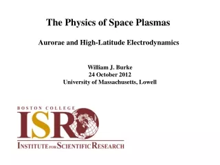
2. Magnetic Storms, Substorms & Generalized Ohm’s Law Lecture 10 • Geomagnetic Storms: (continued ) • Large amplitude FACs and ionospheric conductance sources • The transmission-line analogy • Geomagnetic Substorms: • Growth-phase phenomenology near geostationary altitude • NEXL versus SCW pictures: a perennial controversy • Applications of the Generalized Ohm’s Law: CLUSTER • p = j B => Ingredients of j||

3. Magnetic Storms, Substorms & Generalized Ohm’s Law j||1 dBY dBY dBY j||1 j||2 j||2 dBY dBY dBY j||2 j||2 j||1 j||1

4. Magnetic Storms, Substorms & Generalized Ohm’s Law If ( = 0), then Y Normal Incidence j|| = (1/  0) [YBZ] = (1/ Vsat 0) [t BZ] Vsat  7.5 km/s  1 A/m2  9.4 nT/s J|| = ∫ j|| dY  J|| = (1/  0) [  BZ]1 A/m    BZ = 1256 nT In DMSP-centered coordinates: j|| = Y [PEY -  HEZ] = (1/  0) [YBZ] Oblique Incidence Y [ BZ -  0 ( PEY -  HEZ)] = 0 Where  BZ andEY vary in the same way • P ≈ (1/  0) [  BZ /  EY] • P (mho) ≈   BZ (nT) / 1.256  EY (mV/m)

5. Magnetic Storms, Substorms & Generalized Ohm’s Law During the autumn of 2003 Cheryl Huang and I were studying the distribution and intensities of Region 1 and Region 2 FACs in support of an AFRL effort to model (empirically) the distributions of electric potentials in the global ionosphere. The magnetic storm of 6 April 2000 radically changed our perceptions of stormtime M-I-Tcoupling and the directions of our future research. Huang, C. Y. and W. J. Burke (2004) Transient sheets of field-aligned currents observed by DMSP during the main phase of a magnetic superstorm, JGR, 109, A06303.

6. Magnetic Storms, Substorms & Generalized Ohm’s Law B5 => poleward boundary of auroral oval B2i => ion isotropy boundary: stretched to quasi dipolar field B2e => entry to main plasma sheet: e- energies no loner increase with latitude B1 => equatorward boundary of auroral precipitation.

7. Magnetic Storms, Substorms & Generalized Ohm’s Law • P (mho) ≈   BZ (nT) / 1.256  EY (mV/m) ≈ 25 mho However, the much used equation for Pederson conductance derived from Chatanika ISR where Eave is in keV and FE is in ergs/cm2-s , yield a Pederson conductance of about 5 mho. Something was amiss. But what?

8. Magnetic Storms, Substorms & Generalized Ohm’s Law Note the difference in ion/electron spectral characteristics observed by the SSJ4 ESA on DMSP F4 before and after 20:21:15 UT. It looks as though at 20:21:51UT the electron spectrum became very soft with most of the electron fluxbelow 1 keV. Spectrally this population does not resemble the electron plasma sheet but secondary auroral electrons This phenomenon repeated four timesbefore minimum Dst with relatively small AE enhancemants Found in the late main phase of all major storms with Dst min < -200 nT.

9. Magnetic Storms, Substorms & Generalized Ohm’s Law Transmission line model VAR = Alfvén speed in reflection layer VAS = Alfvén speed at satellite location “Measured” Poynting Flux

10. Magnetic Storms, Substorms & Generalized Ohm’s Law Magnetosphere simulation at 22:00 UT on 6 April 2000 Tsyganenko, N. A., H. J. Singer, and J. C. Kasper, Storm-time distortion of the inner magnetosphere: How severe can it get? J. Geophys. Res., 108 (A5), 1209, 2003.

11. Magnetic Storms, Substorms & Generalized Ohm’s Law During the late main phase of the April 2000 magnetic storm multiple DMSP satellites observed large amplitude FACs with B > 1300 nT). Associated electric fields on the night side were very weak suggesting relatively large P > 25 mho when Robinson formula predicted a small fraction of this amount. We saw a similar effect during the November 2004 storm. Based on strong EUV fluxes from auroral oval Doug Strickland’s model predictedelectron fluxes and energies that were <10% of what DMSP measured No commensurate H measured on ground => Fukushima’s theorem? Do precipitating ions play a significant role in creating and maintaining P[Galand and Richmond, JGR, 2001] ? Does magnetospheric inflation affect the strange particle distributions and intense FACs?

12. Magnetic Storms, Substorms & Generalized Ohm’s Law • Growth phases occur in the intervals between southward turning of IMF BZ and expansion-phase onset. They are characterized by: • Slow decrease in the H component of the Earth’s field at auroral latitudes near midnight. • Thinning of the plasma sheet and intensification of tail field strength. • We consider growth phase electrodynamics observed by the CRRES satellite near geostationary altitude in the midnight sector. - McPherron, R. L., Growth phase of magneto- spheric substorms, JGR, 75, 5592 – 5599, 1970. - Lui, A. T. Y., A synthesis of magnetospheric substorm models, JGR, 96, 1849, 1991. - Maynard, et al., Dynamics of the inner magnetosphere near times of substorm onsets, JGR, 101, 7705 - 7736, 1996. - Erickson et al., Electrodynamics of substorm onsets in the near-geosynchronous plasma sheet, JGR, 105, 25,265 – 25,290, 2000.

13. Magnetic Storms, Substorms & Generalized Ohm’s Law CRRES measurements near local midnight and geostationary altitude during times of isolates substorm growth and expansion phase onsets Ionospheric footprints of CRRES trajectories during orbits 535 (red) and 540 (blue).

14. Magnetic Storms, Substorms & Generalized Ohm’s Law

15. Magnetic Storms, Substorms & Generalized Ohm’s Law

16. Magnetic Storms, Substorms & Generalized Ohm’s Law Erickson et al., JGR 2000: Studied 20 isolated substorm events observed by CRRES. We will summarize one in which the CRRES orbit (461) mapped to Canadian sector LEXO = local explosive onset EXP = explosive growth phase

17. Magnetic Storms, Substorms & Generalized Ohm’s Law

18. Magnetic Storms, Substorms & Generalized Ohm’s Law The Bottom Line: The substorm problem has been with us for a long time. In the 1970s the concepts of near-Earth neutral-line reconnection and disruption of the cross-tail current sheet were widely discussed. To this day there are pitched battles between which has precedence in substorm onset. CRRES data seem to support the substorm current wedge model. During the growth phase the electric field oscillations have little to no associated magnetic perturbations and no measurable field-aligned currents or Poynting flux. (An electrostatic gradient-drift mode that leaves no foot prints on Earth) This ends when E becomes large and Etotal = E0 + E turns eastward and j Etotal < 0. Region becomes a local generator coupling the originally electrostatic to an electromagnetic Alfvén model that carries j|| and S|| to the ionosphere. Pi 2 waves seen when Alfvén waves reach the ionosphere.

19. Magnetic Storms, Substorms & Generalized Ohm’s Law Generalized Ohm’s Law Vasyliunas (1975) wrote the generalized Ohm’s law in the form In ideal MHD the right hand side is zero and E = - V B. With the instrumentation on CLUSTER it is possible to calculate V for ions and measure the components of B and Eto identify regions where the MHD approximation breaks down. Scudder et al 2008 defined a parameter di, e that can be used to identify regions where the gyrotropic approximations for ions and/or electrons breakdown : The symbol w represents the mean thermal speed. If di, e 1 indicates that a species is no longer magnetized. Very useful tool near merging lines! Scudder, J. D., R. D. Holdaway, R. Glassberg, and R. S. Rodriguez (2008), Electron diffusion region and thermal demagnetization, J. Geophys. Res., 113, A10208, doi:10.1029/2008JA013361. Vasyliunas, V. M. (1975), Theoretical models of magnetic field line merging, Rev. Geophys., 13, 303–336, doi:10.1029/RG013i001p00303

20. Magnetic Storms, Substorms & Generalized Ohm’s Law CLUSTER Constellation Launch: July/August 2002 into elliptical orbit with 90o inclination Formation: Variable, tetrahedron most useful for calculating   B. Payload includes sensors to measure: particle distribution, electric and magnetic fields as well as wave spectral characteristics.

21. Magnetic Storms, Substorms & Generalized Ohm’s Law • In a previous lecture we considered Vasyliunas’ formula for j||. • where the symbol V represents the flux tube volume. • Rossi and Olbert ( Chapter 9) show that there are three contributors: • The diamagnetic current jD =   M • The gradient-curvature drift terms jGC

22. Magnetic Storms, Substorms & Generalized Ohm’s Law The total current jT = jD + jGC Thus, jT B For an isotropic plasma Since the divergence of the curl of any vector is zero ( jD) = 0 only the gradient-curvature currents can contribute to j||.