Download
1 / 17
290 likes | 594 Views
CHAPTER 9 Estimation from Sample Data. to accompany Introduction to Business Statistics by Ronald M. Weiers. Chapter 9 - Learning Objectives. Explain the difference between a point and an interval estimate. Construct and interpret confidence intervals:

E N D
CHAPTER 9Estimation from Sample Data to accompany Introduction to Business Statistics by Ronald M. Weiers
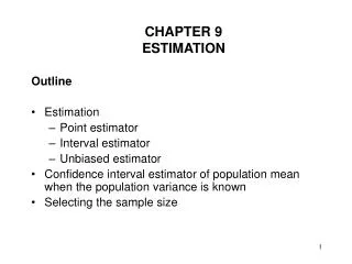
Chapter 9 - Learning Objectives • Explain the difference between a point and an interval estimate. • Construct and interpret confidence intervals: • with a z for the population mean or proportion. • with a t for the population mean. • Determine appropriate sample size to achieve specified levels of accuracy and confidence.
Unbiased estimator Point estimates Interval estimates Interval limits Confidence coefficient Confidence level Accuracy Degrees of freedom (df) Maximum likely sampling error Chapter 9 - Key Terms
x å i x x = n 2 ( x – x ) å 2 2 i = s s n – 1 x successes p p = n trials Unbiased Point Estimates Population Sample Parameter Statistic Formula • Mean, µ • Variance, s2 • Proportion, p
Confidence Interval: µ, s Known where = sample mean ASSUMPTION: s = population standard infinite population deviation n = sample size z = standard normal score for area in tail = a/2
Confidence Interval: µ, s Unknown where = sample mean ASSUMPTION: s = sample standard Population deviation approximately n = sample size normal and t = t-score for area infinite in tail = a/2 df = n – 1
Confidence Interval on p where p = sample proportion ASSUMPTION: n = sample size n•p ³ 5, z = standard normal score n•(1–p) ³5, for area in tail = a/2 and population infinite
Mean: Proportion: Summary: Computing Confidence Intervals from a Large Population
Mean: or Proportion: Converting Confidence Intervals to Accommodate a Finite Population
Interpretation of Confidence Intervals • Repeated samples of size n taken from the same population will generate (1–a)% of the time a sample statistic that falls within the stated confidence interval. OR • We can be (1–a)% confident that the population parameter falls within the stated confidence interval.
s = × e z n 2 2 × s z = n 2 e Sample Size Determination for µ from an Infinite Population • Mean: Note s is known and e, the bound within which you want to estimate µ, is given. • The interval half-width is e, also called the maximum likely error: • Solving for n, we find:
p ( 1 – p ) = × e z n 2 z p ( 1 – p ) = n 2 e Sample Size Determination for p from an Infinite Population • Proportion: Note e, the bound within which you want to estimate p, is given. • The interval half-width is e, also called the maximum likely error: • Solving for n, we find:
An Example: Confidence Intervals • Problem: An automobile rental agency has the following mileages for a simple random sample of 20 cars that were rented last year. Given this information, and assuming the data are from a population that is approximately normally distributed, construct and interpret the 90% confidence interval for the population mean. 55 35 65 64 69 37 88 39 61 54 50 74 92 59 38 59 29 60 80 50
= = x 57 . 9 , s 17 . 384 = = a = df 20 – 1 19 , / 2 0 . 05 = So, t 1 . 729 s 17 . 384 ± × Þ ± × x t 57 . 9 1 . 729 n 20 ± Þ 57 . 9 6 . 721 ( 51 . 179 , 64 . 621 ) A Confidence Interval Example, cont. • Since s is not known but the population is approximately normally distributed, we will use the t-distribution to construct the 90% confidence interval on the mean.
A Confidence Interval Example, cont. • Interpretation: • 90% confident that the interval of 51.179 miles and 64.621 miles will contain the average mileage of the population(m).
An Example: Sample Size • Problem: A national political candidate has commissioned a study to determine the percentage of registered voters who intend to vote for him in the upcoming election. In order to have 95% confidence that the sample percentage will be within 3 percentage points of the actual population percentage, how large a simple random sample is required?
2 2 1 . 96 ( 0 . 5 )( 0 . 5 ) z ( p )( 1 – p ) = = = n 1 , 067 . 1 2 2 e ( 0 . 03 ) A Sample Size Example, cont. • From the problem we learn: • (1 – a) = 0.95, so a = 0.05 and a /2 = 0.025 • e = 0.03 • Since no estimate for p is given, we will use 0.5 because that creates the largest standard error. To preserve the minimum confidence, the candidate should sample n = 1,068 voters.