Chapter 5: CPU Scheduling

1. Chapter 5: CPU Scheduling Adapted to COP4610 by Robert van Engelen

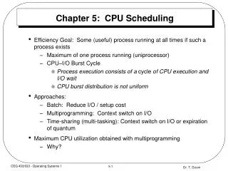
2. Basic Concepts • Maximum CPU utilization is obtained with multiprogramming • Several processes are kept in memory at one time • When a process has to wait, the OS scheduler switches the CPU to another process • Process execution consists of a cycle of CPU execution and I/O wait of varying (but usually short) durations • A process alternates between a CPU burst and an I/O burst • Processes have different CPU-I/O burst distributions

3. Histogram of CPU-burst Times • A CPU-bound process typically has few long CPU burst • An I/O-bound process typically has many short CPU burst • The burst distribution in a system is important for the selection of a CPU-scheduling algorithm (exponential distribution: many more short bursts)

4. CPU Scheduler • Recall that the short-term scheduler selects from among the processes in memory that are ready to execute, and allocates the CPU to one of them through the dispatcher • CPU scheduling decisions may take place when a process: 1. Switches from running to waiting state (e.g. I/O wait) 2. Switches from running to ready state (e.g. interrupt) 3. Switches from waiting to ready (e.g. I/O completion) 4. Terminates • Scheduling under 1 and 4 is nonpreemptive (cooperative) • All other scheduling is preemptive, where processes can be switched at any time without process cooperation • Requires hardware support (timer)

5. Dispatcher • The dispatcher module gives control of the CPU to the process selected by the short-term scheduler • This involves: • Switching context using the context info in the PCB • Switching to user mode • Jumping to the proper location in the user program to restart that program (program counter is in the PCB) • This incurs overhead, the dispatch latency • The time it takes for the dispatcher to stop one process and start another running

6. Dispatch Latency

7. Scheduling Criteria • Criteria to consider for scheduling: • CPU utilization – keep the CPU as busy as possible • Throughput – # of processes that complete their execution per time unit • Turnaround time – amount of time to execute a particular process • Waiting time – amount of time a process has been waiting in the ready queue • Response time – amount of time it takes from when a request was submitted until the first response is produced, not output (for time-sharing environment)

8. Optimization Criteria • When selecting a scheduling algorithm, one or more criteria can be optimized: • Max CPU utilization • Max throughput • Min turnaround time • Min waiting time • Min response time • Not all criteria can be optimized together, because the optimization goals may be (mutually) exclusive • Usually the average measures are optimized

9. P1 P2 P3 0 24 27 30 First-Come, First-Served (FCFS) Scheduling ProcessBurst Time P1 24 P2 3 P3 3 • Suppose that the processes arrive in the order: P1 , P2 , P3 The Gantt Chart for the schedule is: • Waiting time for P1 = 0; P2 = 24; P3 = 27 • Average waiting time: (0 + 24 + 27)/3 = 17 • FCFS is nonpreemptive and usually managed with a FIFO queue

10. P2 P3 P1 0 3 6 30 FCFS Scheduling (Cont.) • Suppose that the processes arrive in the order P2 , P3 , P1 • The Gantt chart for the schedule is: • Waiting time for P1 = 6;P2 = 0; P3 = 3 • Average waiting time: (6 + 0 + 3)/3 = 3 • Much better than previous case • FCFS can lead to the convoy effect, where short processes wait for the long process to get off the CPU

11. Shortest-Job-First (SJF) Scheduling • Associate with each process the length of its next CPU burst • Use these lengths to schedule the process with the shortest time • Two schemes: • nonpreemptive – once CPU given to the process it cannot be preempted until completes its CPU burst • preemptive – if a new process arrives with CPU burst length less than remaining time of current executing process, preempt • This scheme is also known as Shortest-Remaining-Time-First (SRTF) scheduling • SJF is optimal – gives minimum average waiting time for a given set of processes

12. P1 P3 P2 P4 0 3 7 8 12 16 Example of Non-Preemptive SJF Process Arrival TimeBurst Time P1 0.0 7 P2 2.0 4 P3 4.0 1 P4 5.0 4 • SJF according to arrival time (non-preemptive) • Average waiting time = (0 + 6 + 3 + 7)/4 = 4

13. P1 P2 P3 P2 P4 P1 11 16 0 2 4 5 7 Example of Preemptive SJF Process Arrival TimeBurst Time P1 0.0 7 P2 2.0 4 P3 4.0 1 P4 5.0 4 • SJF according to arrival time (preemptive) • Average waiting time = (9 + 1 + 0 +2)/4 = 3 • Better than nonpreemptive SJF

14. Determining Length of Next CPU Burst • Problem: can only estimate the length of the next CPU burst! • Estimate the length using the length of previous CPU bursts, and by using exponential averaging

15. Prediction of the Length of the Next CPU Burst Actual CPU burst time ti Predicted CPU burst time iwith  = 1/2 and 0 = 10

16. Examples of Exponential Averaging • Suppose  =0 • Then n+1 = nRecent history does not count • Suppose  =1 • Then n+1 =  tnOnly the actual last CPU burst counts • If we expand the formula, we get: n+1 =  tn+(1 - ) tn-1+ … +(1 -  )j tn-j+ … +(1 -  )n +1 0 • Since both  and (1 - ) are less than or equal to 1, each successive term has less weight than its predecessor

17. Priority Scheduling • A priority number (integer) is associated with each process • The CPU is allocated to the process with the highest priority • Preemptive • Nonpreemptive • SJF is a priority scheduling where priority is the predicted next CPU burst time • Problem  Starvation (indefinite blocking) – low priority processes may never execute • Solution  Aging – as time progresses increase the priority of the process

18. Round Robin (RR) • Similar to FCFS, but with preemption • Each process gets a small unit of CPU time (time quantum), usually 10-100 milliseconds • After this time has elapsed, the process is preempted and added to the end of the ready queue • If there are n processes in the ready queue and the time quantum is q, then each process gets 1/n of the CPU time in chunks of at most q time units at once • No process waits more than (n-1)q time units • Performance • q large  FIFO • qsmall  q must be large with respect to context switch, otherwise overhead is too high

19. P1 P2 P3 P4 P1 P3 P4 P1 P3 P3 0 20 37 57 77 97 117 121 134 154 162 Example of RR with Time Quantum = 20 ProcessBurst Time P1 53 P2 17 P3 68 P4 24 • The Gantt chart is: • Typically, higher average turnaround than SJF, but better response

20. Time Quantum and Context Switches Smaller time quanta means more context switches

21. Turnaround Time Varies With The Time Quantum Average turnaround time does not necessarily improve with larger quantum

22. Multilevel Queue • Ready queue is partitioned into separate queues: • foreground (interactive) • background (batch) • Each queue has its own scheduling algorithm • foreground – RR • background – FCFS • Scheduling must be done between the queues • Fixed priority scheduling – serve all from foreground then from background • Possibility of starvation • Time slice – each queue gets a certain amount of CPU time which it can schedule amongst its processes; • 80% to foreground in RR • 20% to background in FCFS

23. Multilevel Queue Scheduling

24. Multilevel Feedback Queue • A process can move between the various queues based on process characteristics (aging can be implemented this way) • If a process uses too much CPU time, it is moved to a lower priority queue • If a process waits too long in a lower-priority queue, it is moved to a higher priority queue • Multilevel-feedback-queue scheduler is defined by choosing the following parameters: • How many queues? • Which scheduling algorithms for each queue? • How to determine when to upgrade a process? • How to determine when to demote a process? • How to determine which queue a process will enter when that process needs service?

25. Example of Multilevel Feedback Queue • Three queues: • Q0 – RR with time quantum 8 • Q1 – RR time quantum 16 • Q2 – FCFS • Scheduling • A new job enters queue Q0which is servedFCFS. When it gains CPU, job receives 8 milliseconds. If it does not finish in 8 milliseconds, job is moved to queue Q1 • At Q1 job is again served FCFS and receives 16 additional milliseconds. If it still does not complete, it is preempted and moved to queue Q2

26. Multiple-Processor Scheduling • If multiple CPUs are available, load sharing is possible • CPU scheduling is more complex with multiple CPUs • We assume homogeneous processors within a multiprocessor system • Asymmetric multiprocessing – only one processor accesses the system data structures, alleviating the need for data sharing • Symmetric multiprocessing (SMP) – each processor is self-scheduling using a scheduler that accesses • one common ready queue, or • each processor has a private ready queue

27. Processor Affinity • Migrating a process between processors in SMP causes cache invalidation on the processor being migrated from and cache repopulation on the processor migrated to • Processor affinity keeps a process running on the same processor to reduce cache migration overhead • Soft affinity – OS attempts to keep a process on the same processor • Hard affinity – System call is available to specify that a process is not to migrate to other processors

28. Symmetric Multithreading • SMT (or hyperthreading) provides multiple logical CPUs on a physical CPU • Each logical CPU has own architectural state, i.e. registers, pipelines, mode bits, and interrupt states • Logical CPUs share memory, bus, and cache

29. Thread Scheduling • Local Scheduling – How the threads library decides which user-level thread to put onto an available LWP • The process-contention scope (PCS) scheme • Typically schedules the user-level thread with highest priority (determined by user and thread library) • Supports many-to-many and many-to-one models • Global Scheduling – How the kernel decides which kernel thread to run next • The system-contention scope (SCS) scheme

30. Pthread Scheduling API #include <pthread.h> #include <stdio.h> #define NUM THREADS 5 int main(int argc, char *argv[]) { int i; pthread t tid[NUM THREADS]; pthread attr t attr; /* get the default attributes */ pthread attr init(&attr); /* set the scheduling algorithm to PROCESS or SYSTEM */ pthread attr setscope(&attr, PTHREAD SCOPE SYSTEM); /* set the scheduling policy - FIFO, RT, or OTHER */ pthread attr setschedpolicy(&attr, SCHED OTHER); /* create the threads */ for (i = 0; i < NUM THREADS; i++) pthread create(&tid[i],&attr,runner,NULL);

31. Pthread Scheduling API /* now join on each thread */ for (i = 0; i < NUM THREADS; i++) pthread join(tid[i], NULL); } /* Each thread will begin control in this function */ void *runner(void *param) { printf("I am a thread\n"); pthread exit(0); }

32. Operating System Examples • Solaris scheduling • Windows XP scheduling • Linux scheduling

33. Solaris 2 Scheduling

34. Solaris Dispatch Table

35. Windows XP Priorities

36. Linux Scheduling • Two algorithms: time-sharing and real-time • Time-sharing • Prioritized credit-based – process with most credits is scheduled next • Credit subtracted when timer interrupt occurs • When credit = 0, another process chosen • When all processes have credit = 0, recrediting occurs • Based on factors including priority and history • Real-time • Soft real-time • Posix.1b compliant – two classes • FCFS and RR • Highest priority process always runs first

37. Real-Time Scheduling • Hard real-time systems – required to complete a critical task within a guaranteed amount of time • Soft real-time computing – requires that critical processes receive priority over less fortunate ones

38. The Relationship Between Priorities and Time-slice length

39. List of Tasks Indexed According to Prorities

40. Scheduling Algorithm Evaluation • Evaluation and tuning is based on modeling and simulation • Deterministic modeling – takes a particular predetermined workload and defines the performance of each algorithm for that workload • Queueing models • Simulation • Actual implementation

41. Deterministic Modeling: FCFS vs. SJF vs. RR ProcessBurst Time P1 10 P2 29 P3 3 P4 7 P5 12 • Arrival at time 0 • Consider FCFS, SFJ, and RR with quantum = 10 • Which algorithm(s) give the minimum average waiting time in this case?

42. Deterministic Modeling (cont’d) FCFS: average waiting time is 28 milliseconds SJF (nonpreemptive): average waiting time is 13 milliseconds RR: average waiting time is 23 milliseconds

43. CPU Scheduler Simulation

44. Special Topic: Java Thread Scheduling • JVM uses a preemptive, priority-based scheduling algorithm • FIFO queue is used if there are multiple threads with the same priority

45. Java Thread Scheduling (cont’d) • JVM schedules a thread to run when: • The currently running thread exits the runnable state • A higher priority thread enters the runnable state * Note – the JVM does not specify whether threads are time-sliced or not. The JVM is portable to hardware that may not support preemptive scheduling

46. Time-Slicing • Since the JVM doesn’t ensure time-slicing, the yield() method may be used: while (true) { // perform CPU-intensive task . . . Thread.yield(); } This yields control to another thread of equal priority

47. Thread Priorities PriorityComment Thread.MIN_PRIORITY Minimum Thread Priority Thread.MAX_PRIORITY Maximum Thread Priority Thread.NORM_PRIORITY Default Thread Priority Priorities may be set using setPriority() method: setPriority(Thread.NORM_PRIORITY + 2);

48. End of Chapter 5