Download

1 / 10
100 likes | 211 Views
A canopy model of mean winds through urban areas. O. COCEAL and S. E. BELCHER University of Reading, UK. Motivation. urban areas have an effect on mesoscale weather processes local winds within urban areas need to be considered for local weather forecasts and building design applications

E N D
A canopy model of mean winds through urban areas O. COCEAL and S. E. BELCHER University of Reading, UK
Motivation • urban areas have an effect on mesoscale weather processes • local winds within urban areas need to be considered for local weather forecasts and building design applications • urban air quality is becoming an issue of increasing concern, and the processes controlling mixing and transport of pollutants have a wide range of scales
Motivation • The dynamical effect of urban areas is usually represented in NWP at present through a simple roughness length. Problems: • gives no information on the mixing and transport within the urban canopy • a roughness length can be defined only when the wind profile near the surface is logarithmic, sometimes difficult to measure • not practical, and not desirable, to compute the flow around every building in a big city • Need a more sophisticated method of representing the dynamical effects of urban areas than a roughness length.
Formulation of the Model • By averaging the governing equations, firstly over time, and secondly over a volume • The averaging volume should be very thin in the vertical, and large enough in the horizontal to include a number of canopy elements • Prognostic variables then have three components, eg. the streamwise velocity u are : time- and space-averaged velocity, mean velocity : spatial variation of the time-mean flow around individual roughness elements : the turbulent fluctuation
Formulation of the Model • To calculate the mean wind vector Ui(x, y, z) , by solving the time- and space-averaged momentum equations: • Three new terms: : spatially averaged Reynolds stress, momentum transport due to turbulent-velocity fluctuations : dispersive stress, momentum transport by the spatial deviations from the spatially averaged wind : canopy-element drag, spatially averaging the localized drag due to individual roughness elements • The drag term is important through the whole volume of the canopy, the dispersive stress can be neglected, the urban canopy model is completed on parametrizing the drag and the turbulent stress
Parametrization of the canopy-element drag • canopy drag length-scale • Lc is determined by the geometry and layout of the obstacles, as expressed by the parameters roughness density, air fractional volume in the canopy and drag coefficient • The drag coefficient has a dependence on the shape of the obstacles. • cd(z) is the sectional drag coefficient that relates the drag at height z to the average wind speed at that height, differs from the depth-integrated drag coefficient Cdh .
Reynolds stress parametrization • The Prandtl mixing-length model is used to represent the spatially averaged turbulent stress : shear rate lmrepresents a spatially averaged turbulence integral length-scale, which is expected to depend on characteristics of the canopy, such as the obstacle density • If the canopy is very sparse the turbulence structure of the boundary layer is not much affected by the canopy; when the canopy is denser the boundary-layer eddies above the canopy are blockedby the strong shear layer that forms near the top of canopy.
Flow within and above a homogeneous canopy • When the canopy is sufficiently extensive the winds both within and above are adjusted, within the canopy the dynamical balance is between the vertical stress gradient and the drag force. • Profiles for canopies with different values of Lc and h, but with the same value of Lc/h, collapse onto each other, the plots are nearly overlaped.
Conclusions • This model captures the variations in the spatially averaged mixing and transport induced by changes in density and type of urban roughness elements. • Important differences exist in the way the drag and mixing are parametrized. • Only a few parameters are needed to initialize the model, and the morphological parameters are relatively straightforward to estimate. • The urban canopy model compares well with wind tunnel and field measurements of the profiles of spatially averaged wind above and within regular arrays of cubical obstacles.
Discussion • The heterogeneity over a wide range of length-scales? • The difference between this urban canopy model and the quasi-linear model of BJH? • The dispersive stress term importance and affection?