Download
1 / 71
980 likes | 1.6k Views
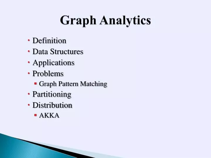
Graph Analytics . Definition Data Structures Applications Problems Graph Pattern Matching Partitioning Distribution AKKA. Fast review on Graph and graph theory. Definition: A "graph" is a collection of " vertices" or "nodes" " edges " that connect pairs of vertices.

E N D
Graph Analytics • Definition • Data Structures • Applications • Problems • Graph Pattern Matching • Partitioning • Distribution • AKKA
Fast review on Graph and graph theory Definition: • A "graph" is a collection of • "vertices" or "nodes" • " edges "that connect pairs of vertices. • A graph may be undirected, meaning that there is no distinction between the two vertices associated with each edge, or its edges may be directed from one vertex to another 2 1 3 2 1 3
Applications • The link structure of a website could be represented by a directed graph. The vertices are the web pages available at the website and a directed edge from page A to page B exists if and only if A contains a link to B. Mathematical PageRanks for a simple network, expressed as percentages. (Google uses a logarithmic scale.) Page C has a higher PageRank than Page E, even though there are fewer links to C; the one link to C comes from an important page and hence is of high value. • graph theory is also used to study molecules in chemistry and physics. In condensed matter physics, the three dimensional structure of complicated Simulated atomic structures. • Image Processing, crime detection • Antology • …
Graph-theoretic data structures The data structure used depends on both the graph structure and the algorithm used for manipulating the graph. Theoretically one can distinguish between list and matrix structures but in concrete applications the best structure is often a combination of both. • Liststructures are often preferred for sparse graphs as they have smaller memory requirements. • Matrixstructures on the other hand provide faster access for some applications but can consume huge amounts of memory.
List • Incidence list The edges are represented by an array containing pairs (tuples if directed) of vertices (that the edge connects) and possibly weight and other data. Vertices connected by an edge are said to be adjacent. ((a,b),(c,d),…) • Adjacency list Much like the incidence list, each vertex has a list of which vertices it is adjacent to. This causes redundancy in an undirected graph: for example, if vertices A and B are adjacent, A's adjacency list contains B, while B's list contains A. Adjacency queries are faster, at the cost of extra storage space.
Matrix • Incidence matrix The graph is represented by a matrix of size |V | (number of vertices) by |E| (number of edges) where the entry [vertex, edge] contains the edge's endpoint data (simplest case: 1 - incident, 0 - not incident). e1 e2 e3 e4 1 2 3 4 • Adjacency matrix This is an n by n matrix A, where n is the number of vertices in the graph. If there is an edge from a vertex x to a vertex y, then the element is 1 (or in general the number of xy edges), otherwise it is 0. In computing, this matrix makes it easy to find subgraphs, and to reverse a directed graph.
Matrix • Distance matrix A symmetric n by n matrix D, where n is the number of vertices in the graph. The element is the length of a shortest path between x and y; if there is no such path = infinity. It can be derived from powers of A
Matrix • Laplacianmatrix or "Kirchhoff matrix" or "Admittance matrix" This is defined as D − A, where D is the diagonal degree matrix. It explicitly contains both adjacency information and degree information. (However, there are other, similar matrices that are also called "Laplacian matrices" of a graph.)
Problems in graph theory • Enumeration • Subgraphs, induced subgraphs, and minors • Graph coloring • Route problems • Network flow • Visibility graph problems • Covering problems • Graph classes
Enumeration Enumeration describes a class of combinatorial enumeration problems in which one must countundirected or directed graphs of certain types, typically as a function of the number of vertices of the graph. Application: • Enumeration of molecules has been studied for over a century and continues to be an active area of research. • The typical approach to enumerating chemical structures has been based on constructive assembly. It is list of all free trees on 2,3,4 labeled vertices: tree with 2 vertices, trees with 3 vertices, trees with 4 vertices.
Subgraphs, induced subgraphs, and minors 2.1. Subgraphs: A common problem, called the subgraph isomorphism problem, is finding a fixed graph as a subgraphin a given graph. The subgraph isomorphism problem is a computational task in which two graphs G and Qare given as input, and one must determine whether G contains a subgraphthat is isomorphic to Q. Subgraph isomorphism is a generalization of both the maximum clique problem and the problem of testing whether a graph contains a Hamiltonian cycle, and is therefore NP-complete. • clique problem: Finding the largest complete graph is called the clique problem. The term "clique" and the problem of algorithmically listing cliques both come from the social sciences, where complete subgraphs are used to model social cliques, groups of people who all know each other. In computer science, the clique problem refers to any of the problems related to finding particular complete subgraphs("cliques") in a graph, i.e., sets of elements where each pair of elements is connected.
Subgraphs, induced subgraphs, and minors 2.2 Induced subgraphs: some important graph properties are hereditary with respect to induced subgraphs, which means that a graph has a property if and only if all induced subgraphs also have it. Finding maximal induced subgraphs of a certain kind is also often NP-complete. • Finding the largest edgeless induced subgraph, or independent set, called the independent set problem • An independent set or stable set is a set of vertices in a graph, no two of which are adjacent. That is, it is a set I of vertices such that for every two vertices in I, there is no edge connecting the two. The size of an independent set is the number of vertices it contains. The graph of the cube has six different maximal independent sets, shown as the red vertices.
Subgraphs, induced subgraphs, and minors 2.3. Minors: The minor containment problem, is to find a fixed graph as a minor of a given graph. A minor or subcontraction of a graph is any graph obtained by taking a subgraph and contracting some (or no) edges. Many graph properties are hereditary for minors, which means that a graph has a property if and only if all minors have it too • A graph is planar if it contains as a minor neither the complete bipartite graph (Three-cottage problem) nor the complete graph . Graph can be drawn in such a way that no edges cross each other. Such a drawing is called a plane graph or planar embedding of the graph. • Three-cottage problem: water, gas, and electricity, the (three) utilities problem: Suppose there are three cottages on a plane and each needs to be connected to the gas, water, and electric companies. Using a third dimension or sending any of the connections through another company or cottage is disallowed. Is there a way to make all nine connections without any of the lines crossing each other? The utility graph K3,3 K3,3drawn with only one crossing.
Graph coloring Many problems have to do with various ways of coloring graphs, for example: • The four-color theorem: In mathematics, the four color theorem, or the four color map theorem states that, given any separation of a plane into contiguous regions, producing a figure called a map, no more than four colors are required to color the regions of the map so that no two adjacent regions have the same color. • The strong perfect graph theorem: In graph theory, a perfect graph is a graph in which the chromatic number of every induced subgraph equals the size of the largest clique of that subgraph. Perfect graphs are the same as the Berge graphs, graphs that have no odd-length induced cycle or induced complement of an odd cycle. The chromatic polynomial counts the number of ways a graph can be colored using no more than a given number of colors. The Paley graph of order 9, colored with three colors and showing a clique of three vertices. In this graph and each of its induced subgraphs the chromatic number equals the clique number, so it is a perfect graph.
Graph coloring • The total coloring conjecture (unsolved): In graph theory, total coloring is a type of coloring on the vertices and edges of a graph. When used without any qualification, a total coloring is always assumed to be proper in the sense that no adjacent vertices, no adjacent edges, and no edge and its endvertices are assigned the same color. The total chromatic number χ″(G) of a graph G is the least number of colors needed in any total coloring of G. • The Erdős–Faber–Lovász conjecture (unsolved) • The list coloring conjecture (unsolved) • The Hadwiger conjecture (graph theory) (unsolved)
Route problems 4.1. Hamiltonian path and cycle problems: Hamiltonian path problem and the Hamiltonian cycle problem are problems of determining whether a Hamiltonian path or a Hamiltonian cycle exists in a given graph • Hamiltonian path: a Hamiltonian path is a path in an undirected graph that visits each vertex exactly once. A Hamiltonian cycle (or Hamiltonian circuit) is a Hamiltonian path that is a cycle 4.2. Minimum spanning tree: In an undirected graph, a spanning tree of that graph is a subgraphthat connects all the vertices together. 4.3. Route inspection problem : route inspection problem is to find a shortest closed path or circuit that visits every edge of a (connected) undirected graph
Route problems 4.4. Seven Bridges of Königsberg: The problem was to find a walk through the city that would cross each bridge once and only once 4.5. Shortest path problem: the shortest path problem is the problem of finding a path between two vertices (or nodes) in a graph such that the sum of the weights of its constituent edges is minimized. 4.6. Steiner tree: problem in combinatorial optimization, which may be formulated in a number of settings, with the common part being that it is required to find the shortest interconnect for a given set of objects 4.7. Three-cottage problem 4.8. Traveling salesman problem : Given a list of cities and their pairwise distances, the task is to find the shortest possible route that visits each city exactly once and returns to the origin city
Graph pattern matching • Graph pattern matching is often defined in terms of subgraphisomorphism, an NP-complete problem. To lower its complexity, various extensions of graph simulation have been considered instead. Given a pattern graph Q and a data graph G, it is to find all subgraphs of G that match Q. input images detected features one-shot matching (26 true) gressivematching (159 true)
Graph pattern matching • Isomorphism: In graph theory, an isomorphism of graphs G and Q is a bijection between the vertex sets of G and Q ( Q G ) such that any two vertices u and v of G are adjacent in G if and only if ƒ(u) and ƒ(v) are adjacent in Q • A bijection(or bijective function or one-to-one correspondence) is a function giving an exact pairing of the elements of two sets.
Graph Simulation As observed, it is often too restrictive to catch sensible matches, as it requires matches to have exactly the same topology as a pattern graph. These hinder its applicability in emerging applications such as social networks and crime detection. • Simple Simulation : denoted by Q ≺ G, S ⊆ VQ × V , where VQand V are the set of nodes in Q and G, respectively, such that • for each (u, v) ∈ S, u and v have the same label; • for each node u in Q, there exists v in G such that • (u, v) ∈ S, • for each edge (u, u’)in Q, there exists an edge (v, v’) in G such that (u’, v’)∈ S. (same children) G Q 200 100 Book Book TE TE TE ST 4 1 4 1 300 Book 2 2 Book ST ST 5 5 Book 3 3 ST ST
Graph Simulation • Dual simulation: denoted by Q ≺D G, • if Q ≺ G with a binary match relation S ⊆ Vq × V , • for each pair (u, v) ∈ S and each edge (u2, u) in Eq, there exists an edge (v2, v) in E with (u2, v2) ∈ S. (same children and same parents) Q G Book TE TE 200 100 4 1 TE ST 1 Book 2 2 Book ST 300 ST 5 5 3 Book 3 ST ST
0 A G 1 B Q Simple Simulation • More Example of Simple and Dual Simulation 0 A 2 100 B A 1 B 3 B 200 B 2 8 B A 4 7 B K 3 5 B B 0 Dual Simulation 8 A A 4 B 1 B 5 B 9 3 A B 6 D 8 A 4 B
Simple Simulation Q G • More Example of Simple and Dual Simulation 10 1 A A C B C B 3 30 2 20 4 D D D 40 5 E F 8 9 E F F E 50 60 6 7 E F 10 11
Graph Simulation • Strong simulation: Define strong simulation by enforcing two conditions on simulation : duality and locality. Balls. For a node v in a graph G and a non-negative integer r, the ball with center v and radius r is a subgraph of G, denoted by ˆG[v, r], such that • for all nodes v in ˆG[v, r], the shortest distance dist(v, v) ≤ r, • it has exactly the edges that appear in G over the same node set. denoted by Q ≺DL G, if there exist a node v in G and a connected subgraphGsof G such that • Q ≺DGs, with the maximum match relation S; • Gsis exactly the match graph w.r.t. S • Gsis contained in the ball ˆG[v, dQ], where dQis the diameter of Q. P P P Q G 2 1 3 2 P P P 100 3 2 1 P 4 4 P P P 3 2 1 4 P P 200 P 1 3 P P P 4 P
G Q • More Example of Simple and Dual Simulation 0 0 0 A A A 100 A 0 A 1 1 1 1 B B B B 200 B 2 2 2 2 A A A A 3 3 3 3 B B B B 4 4 4 4 A A A A 5 5 5 B B B B 5 6 6 6 B B A 6 B
DM1 DM2 DM SE1 HR1 Bio2 Bio1 SE2 HR2 Al1 AI1 AIk Bio DM1 Bio3 DMk1 Bio4 Al2 AI HR SE Graph Simulation Example 1: the Bio has to be recommended by: • an HR person; • an SE, i.e., the Bio has experience working with SEs; • The SE is also recommended by an HR person • a data mining specialist (DM), as data mining techniques are required for the job. • there is an artificial intelligence expert (AI) who recommends the DM and is recommended by a DM.
Optimization Techniques We next present optimization techniques for algorithm Match, by means of • Query minimization • Dual simulation filtering • Connectivity pruning • Query minimization: We say that two pattern graphs Q and Q’ are equivalent, denoted by Q ≡ Q’, if they return the same result on any data graph. A pattern graph Q is minimum if it has the least size |Q| (the number of nodes and the number of edges) among all equivalent pattern graphs. R R B1 B2 A B1 A D1 C1 D1 D2 C2 C1
Optimization Techniques • Dual simulation filtering. Our second optimization technique aims to avoid redundant checking of balls in the data graph. Most algorithms of graph simulation recursively refine the match relation by identifying and removing false matches. So, we compute the match relation of dual simulation first, and then project the match relation on each ball to compute strong simulation. This both reduces the initial match set sim(v) for each node v in Q and reduces the number of balls . Indeed, if a node v in G does not match any node in Q, then there is no need to consider the ball centered at v. • The removal process on a ball only needs to deal with its border nodes and their affected nodes. P P3 P2 P1 P3 P1 P4 P4 P’ G Q
Optimization Techniques • Connectivity pruning. In a ball, only the connected component containing the ball center v needs to be considered. Hence, those nodes not reachable from v can be pruned early. B2 A2 B1 A1 Q B2 A2 C B1 A1 G
defhhk (g: Graph, q: Graph): Unit = { valsim = HashMap[Int, Set[Int]]() q.vertices.foreach ( u => { varlis = Set[Int]() g.vertices.filter( w => g.label(w) == q.label(u)).foreach ( wp => lis += wp ) sim += u -> lis }) var flag = true while (flag) { flag = false for (u <- q.vertices; w <- sim(u); v <- q.post(u) if (g.post(w) & sim(v)).isEmpty ) { sim(u) -= w flag = true } for (u <- q.vertices; w <- sim(u); v <- q.pre(u) if (g.post(w) & sim(v)).isEmpty ) { sim(u) -= w flag = true } //for } //while }
For all v € G If post (v) =0 then sim(v) = { u € Q | <<u>> = <<v>>} Else sim(v) = { u € Q | <<u>> = <<v>> and post (u) ≠ 0} Remove (v) := pre ( G) – pre (sim(v)) While there is v € G , remove(v) ≠ 0 for all u € pre(v) for all w € remove (v) if w € sim (u) sim (u) = sim (u) – {w} for all w’ € pre (w) if post(w’) ᴨsim (u) = 0 then remove (u) := remove (u) ᴜ {w’} remove (v) = 0 • Sim ( D) = { D1,D2} • Remove (v) := pre ( G) – pre (sim(v)) • Remove (D) = {A1,B1,C1,D1,C2,C3} – {C2,C3,A1,B1} = {C1,D1} • For u -> Pre(D) = { C,A} • for w -> Remove (D) = {C1,D1} • if w €sim(C) = {C1,C2,C3,A1} => sim (C) = {C1,C2,C3}–{C1} • for all w’ € pre (w) = {A1} • if post(A1) ᴨSim(C) = {C2,C3} ==0 (False) C2 D2 A1 A C3 C1 B1 D1 B C D H G
Graph Simulation Home work: Pattern Qis looking for papers on social networks (SN) cited by papers on databases (db), which in turn cite papers on graph theory (graph). Fined the pattern graph and all Isomorphism, Simple simulation, Dual simulation and strong simulation match graph of that with given graph G DB1 DB2 DB3 SN3 SN1 Graph2 Graph1 SN2 SN4
Goals of Partitioning • The balance constraint: • Balance computational load such that each processor has the same execution time • Balance storage such that each processor has the same storage demands • Minimum edge cut: • Minimize communication volume between subdomains, along the edges of the mesh 4-cut 5-cut Example 3-way partition with edge-cut = 9
Distributed Graph Pattern Matching We now define the graph pattern matching problem in a distributed setting. Given pattern graph Q, and fragmented graph F = (F1, . . ., Fk) of data graph G, in which each fragment Fi = (G[Vi], Bi) (i ∈ [1, k]) is placed at a separate machine Si, the distributed graph pattern matching problem is to find the maximum match in G for Q, via graph simulation. F1 = (G[V1], {BPM1 , BSA1 }), V1 = {PM1, BA1} BPM1 = {BA1 : 2}, BSA1 = {SD1 : 2}, F2 = (G[V2], ∅), V2 = {SA1, ST1}, F3 = (G[V3], {BPM2}), V3 = {PM2,BA2,UD1}, BPM2 = {SA2 : 4} and BSA2 = {SDh : 5}, F4 = (G[V4], {BSA2 }), V4 = {SA2}, F5 = (G[V5], ∅), V5 = {SD1, ST1, . . . , SDh, STh}, F4 F3 F2 F1 PM2 PM SA2 PM1 BA1 SA BA UD UD1 BA2 SD1 SA1 F5 SD ST ST1 STn SD1 SDn
Distributed Graph Pattern Matching Partial match. A binary relation R ⊆ Vq × Vi is said to be a partial match if • (1) for each (u, v) ∈ R, u and v have the same label; • (2) for each edge (u, u’) in Eq, • (a) there exists a node v’ ∈ Bv in Bi having the same label as u’ if v is a boundary node • (b) there exists an edge (v, v’) in G[Vi] such that (u’, v’) ∈ R Pair (SA, SA1) is in the maximum partial match PM1 in fragment F1 for Q. However, it does not belong to the maximum match M in G for Q.Consider pattern graph Q1 and data graph G1 , and the partial match results . (1) For node SA1, its only child SD1 is located in fragment F2. The partial match SD1 is empty. Hence, a false match decision is sent back to machine S1, and this further helps determine that (SA,SA1) is a false match. (2) For node SA2, its only child SDn is located in fragment F5. The subgraph F5 contains no boundary nodes, and SDn belongs to F5. Hence, a true match decision is sent back to machine S4, and this further helps determine that (SA,SA2) is a true match. After these are done, fragment F3 is the only part of G that needs to be further evaluated. To check the matches in F3, we simply ship fragment F4 to machine S3. F3 F4 F2 PM2 F1 PM1 BA1 PM SA2 UD1 BA2 SA BA UD SD1 SA1 F5 SD ST ST1 STn SD1 SDn
Q G D, E, F 1 D A 5 B 2 C • Go for each matched label vertex and create the ball. with d=4 (L=2) 3 D F E 6 7 12 4 4 D D D D 40 E F 8 9 E F 8 9 F E F 50 60 E 10 11 E F 10 11 D 12 D 4 5 D F 8 9 E F E 6 7 E F 10 11
The Problem • Correct highly scalable systems. • Fault tolerant system that self heals. • Truly scalable systems. ………. Using state of the art tools.
Vision • …. Simpler • Concurrency • Scalability • Fault Tolerance • With a single unified • Programming Model • Runtime Service
Where is Akka used? • Finance • Stock trend analysis and simulation. • Event Driven Messaging Systems. • Betting and Gaming • Massive multiplayer online gaming • High throughput and transactional betting. • Telecom • Streaming media network gateways. • Simulation • 3 D Simulation Engine. • Ecommerce • Social Media Community Sites.
What is “Actor Model” • Incomputer science, the Actor model is a mathematical model of concurrent computation that treats "actors" as the universal primitives of concurrent digital computation: in response to a message that it receives, an actor can make local decisions, create more actors, send more messages, and determine how to respond to the next message received.
AKKA is a toolkit and runtime for building highly concurrent distributed and fault tolerant even driven application on the JVM • Parallism • Concurrency Event Driven Actor Behavior State
Actors class object Tick class Counter extends Actors { Var counter =0 Defreceive ={ Case tick => Counter += 1 Println (counter) } }
Create Actors Val counter = actorOf[Counter] Counter is an ActorRef
Send ! Counter ! tick
Send !!! val future=actor !!! Message future.await val result = future.result
Reply Class SomeActor extends Actor { def receive = { Case User(name) => Self.reply("Hi" + name) } }
Hot Swap Self become{ Case NewMessage => ……. }