Download
1 / 58
1.11k likes | 1.78k Views
Experimental design. Experimentation. An experiment imposes a treatment on a group of objects or subjects in the interest of observing the response. Treatment. In experiments, a treatment is something that researchers administer to experimental units.

E N D
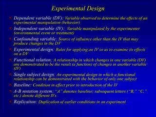
Experimentation • An experimentimposes a treatment on a group of objects or subjects in the interest of observing the response.
Treatment • In experiments, a treatment is something that researchers administer to experimental units. • For example, a corn field is divided into four, each part is 'treated' with a different fertilizer to see which produces the most corn; • a teacher practices different teaching methods on different groups in her class to see which yields the best results; • a doctor treats a patient with a skin condition with different creams to see which is most effective.
Levels of treatment • Treatments are performed to experimental units by 'level', where level implies amount or magnitude. • For example, if the experimental units were given 5mg, 10mg, 15mg of a medication, those amounts would be three levels of the treatment.
Factor • A factor is a general type or category of treatments. • A factor of an experiment is a controlled independent variable; • a variable whose levels are set by the experimenter. • Different treatments constitute different levels of a factor. • For example, three different groups of runners are subjected to different training methods. • The runners are the experimental units (or subjects, or samples), the training methods, the treatments, where the three types of training methods constitute three levels of the factor 'type of training'.
The Completely Randomized Design (CRD) • The CRD is the simplest of all designs. It is equivalent to a t-test when only two treatments are examined.
Field marks: • Replications of treatments are assigned completely at random to independent experimental subjects.
Sample layout • Different colors represent different treatments. There are 4 (A-D) treatments with 4 replications (1-4) each.
A1B1C1A2 • D1 A3 D2 C2 • B2 D3 C3B3 • C4A4B4 D4
Experimental design Fine root production of Fertilization experiment Treatment: Concentration of Fertilization Fine root production (year6)
RANDOMIZED COMPLETE BLOCK DESIGN (RCBD) • Description of the Design • • Probably the most used and useful of the experimental designs. • • Takes advantage of grouping similar experimental units into blocks or replicates. • • The blocks of experimental units should be as uniform as possible. • • The purpose of grouping experimental units is to have the units in a block as uniform as possible so that the observed differences between treatments will be largely due to “true” differences between treatments.
Randomization Procedure • • Each replicate is randomized separately. • • Each treatment has the same probability of being assigned to a given experimental unit within a replicate. • • Each treatment must appear at least once per replicate.
Example • Given four fertilizer rates applied to ‘Amidon’ wheat and three replicates of each treatment. • Rep 1 Rep 2 Rep 3Rep 4 • A B A A A=0 kg N/ha • D A B B B=50 kg N/ha • C D C C C=100 kg N/ha • B C D D D=150 kg N/ha
Advantages of the RCBD • 1. Generally more precise than the CRD. • 2. No restriction on the number of treatments or replicates. • 3. Some treatments may be replicated more times than others. • 4. Missing plots are easily estimated. • 5. Whole treatments or entire replicates may be deleted from the analysis. • 6. If experimental error is heterogeneous, valid comparisons can still be made.
Disadvantages of the RCBD • 1. Error df is smaller than that for the CRD (problem with a small number of treatments). • 2. If there is a large variation between experimental units within a block, a large error term may result (this may be due to too many treatments). • 3. If there are missing data, a RCBD experiment may be less efficient than a CRD • NOTE: The most important item to consider when choosing a design is the uniformity of the experimental units. • RCBD – No Sampling
Split Plot Experiment • One of the most common mixed models is the split-plot design. • The split-plot design involves two experimental factors, A and B. • Levels of A are randomly assigned to whole plots (main plots), and levels of B are randomly assigned to split plots (subplots) within each whole plot. • The subplots are assumed to be nested within the whole plots so that a whole plot consists of a cluster of subplots and a level of A is applied to the entire cluster. • The design provides more precise information about B than about A, and it often arises when A can be applied only to large experimental units.
The hypothetical data set analyzed in this example was created as a balanced split-plot design with the whole plots arranged in a randomized complete-block design. The response variable Y represents crop growth measurements. • The variable A is a whole plot factor that represents irrigation levels for large plots, and the subplot variable B represents different crop varieties planted in each large plot. • The levels of B are randomly assigned to split plots (subplots) within each whole plot. The data set Split contains the whole plot factor A, split plot factor B, response Y, and blocking factor Block. • Using the Mixed Models task, you can estimate variance components for Block, A*Block, and the residual and automatically incorporate correct error terms into the tests for fixed effects.
What Is a Split-Plot Design? • In simple terms, a split-plot experiment is a blocked experiment, where the blocks themselves • serve as experimental units for a subset of the factors. • Thus, there are two levels of experimental units. The • blocks are referred to as whole plots, while the experimental units within blocks are called split plots, split units, or subplots. Corresponding to the two levels of experimental units are two levels of randomization. • One randomization is conducted to determine the assignment of block-level treatments to whole plots. • Then, as always in a blocked experiment, a randomization • of treatments to split-plot experimental units occurs within each block or whole plot.
Split-plot designs were originally developed by • Fisher (1925) for use in agricultural experiments. • As a simple illustration, consider a study of the effects • of two irrigation methods (factor A) and two fertilizers • (factor B) on yield of a crop, using four available • fields as experimental units. • In this investigation, it is not possible to apply different irrigation methods • (factor A) in areas smaller than a field, although different • fertilizer types (factor B) could be applied in relatively small areas. • For example, if we subdivide each whole plot (field) into two split plots, each of the two fertilizer types can be applied once within each • whole plot, as shown in Figure 1. In this split-plot • design, a first randomization assigns the two irrigation • types to the four fields (whole plots); then within • each field, a separate randomization is conducted to • assign the two fertilizer types to the two split plots within each field.
Why Use Split-Plot Designs? • In this paper, we advocate greater consideration of split-plot experiments for three reasons: cost, efficiency, and validity. In this section, we discuss each of these advantages in turn.
Cost • The cost of running a set of treatments in split-plot order is generally less than the cost of the same experiment when completely randomized. • As Ganju and Lucas (1997, 1998, 2005) have noted, a properly implemented completely randomized design (CRD) requires that all factors must be independently reset with each run. If a factor level does not change from one run to the next and the factor level is not reset (e.g., by changing its level and then changing it back), inadvertent split plotting occurs.
Efficiency • Split-plot experiments are not just less expensive to run than completely randomized experiments; • they are often more efficient statistically. • Ju and Lucas (2002) show that, with a single hard-to-change factor or a single easy-to-change factor, use of a split-plot layout leads to increased precision in the estimates for all factor effects except for whole-plot main effects.
Validity • Completely randomized designs are prescribed frequently in industry, but are typically not run as such in the presence of hard-to-change factors. • One of two shortcuts may be taken by the experimenter in the interest of saving time or money, i.e., • 1. A random-run-order (RRO) design—alternately referred to as a random-not-reset (RNR) design—is utilized.
in this case, • the order of treatments is randomized, but the factor levels are not reset with each run of the experiment, or perhaps all factors, except the hard-to-change factors are reset. • Not resetting the levels of the hard-to-change factor leads to a correlation between adjacent runs. Statistical tests that do not consider these correlations will be biased
How to Choose a Split-Plot Design • Choosing a “best” split-plot design for a given design scenario can be a daunting task, even for a professional statistician. • Facilities for construction of split-plot designs are not as yet generally available in software packages (with SAS/JMP being one exception).
we discuss the choice of split-plot designs in five areas: • (1) two-level full factorial designs; • (2) two-level fractional factorial designs; • (3) mixture and response surface designs; (4) split-plot designs for robust product experiments; • (5) optimal designs.
Full Factorial Split-Plot Designs • Construction of single replicates of a two-level full factorial designs is straightforward. • In this case, a completely randomized design in the whole-plot factors is conducted and, within each whole plot, a completely randomized design in the split-plot factors is also conducted.
Fractional Factorial Split-Plot Designs • If a full factorial split-plot design is too large, consideration of a fractional factorial split-plot (FFSP)
Split-Plot Designs for Robust ProductExperiments • The purpose of robust product experiments is to identify settings of product-design factors, sometimes termed product-design parameters that lead to products or processes that are insensitive to the effects of uncontrollable environmental factors. • As illustrated by Box and Jones (1992), product-design parameters for a cake mix might be the amount of flour, shortening, and egg powder contained in the mix. Uncontrollable environmental factors include the baking time and baking temperature used by the consumer to produce the cake.
Split-Plot Designs for Response SurfaceExperiments • Relatively little research has been conducted with regard to the construction of split-plot designs for response surface experiments. • Recall that, in a response surface experiment, we are typically interested in estimating a response model comprised of all first- and second-order polynomial terms.
Optimal Split-Plot Designs • A general approach to the problem of constructing split-plot designs is provided by the optimal-design approach. • The general approach is as follows: • 1. Specify the number of whole plots, nw. • 2. Specify the number of split plots per whole plot, ns. • 3. Specify the response model, f (w, s). • 4. Specify a prior estimate of the variance ratio, d. • 5. Use computer software to construct the design • for steps 1 through 4 • 6. Study the sensitivity of the optimal design to • small changes in d, nw, and ns.
Example • SPLIT PLOT DESIGN • 2 Main Plot Treatments (1, 2) • 2 Sub Plot Treatments (A, B) • 4 Blocks • Block 1 • 2 A 2 B 1 B 1 A • Block 2 • 1 B 1 A 2 B 2 A • Block 3 • 1 B 1 A 2 A 2 B • Block 4 • 2 A 2 B 1 A 1 B
Sample layout: • Different colors represent different treatments; each horizontal row represents a block. • Plot colors represent assignment of main effects or treatments; • top plant colors split plots; bottom colors split-split treatments. • There are 3 blocks (I-III) each of 2 main treatments (A & B) split into 2 treatments (1 & 2) and further split into 3 treatments (a-c) in split-split plots.
Nested Designs • I. Why • Sometimes it is difficult or impossible to cross all of the factors of interest in an experimental design. • The experimenter may then choose to use a fractional factorial design or latin square. • If each level of one factor is paired with only one level of another factor, then the first factor is said to be nested within the second factor.
Examples • A. The effect on individual teachers of school district policies. Teachers are nested within school districts: T(D). • District • A B C • Teacher: T1T2 T3T4 T5T6
If this were a completely crossed design, each teacher would work in each district; i.e., the cells in the following table would be filled. As it is, there are observations in only 6 (see x's) cells. • District • A B C • T1 x • T2 x • T3 x • T4 x • T5 x • T6 x
B. The effect of teacher training in different school districts on students' accomplishments. • District • A B C Teacher T1T2T3T4T5 T6 • S1 S4 S7 S10 S13 S16 Students S2 S5 S8 S11 S14 S17 • S3 S6 S9 S12 S15 S18
Nested Designs Study vs Control Site
Nested Experiments • In some two-factor experiments the level of one factor , say B, is not “cross” or “cross classified” with the other factor, say A, but is “NESTED” with it. • The levels of B are different for different levels of A. • For example: 2 Areas (Study vs Control) • 4 sites per area, each with 5 replicates. • There is no link from any sites on one area to any sites on another area.
Study Area (A) Control Area (B) S1(A) S2(A) S3(A) S4(A) S5(B) S6(B) S7(B) S8(B) X X X X X X X X X X X X X X X X X X X X X X X X X X X X X X X X X X X X X X X X X = replications Number of sites (S)/replications need not be equal with each sites. Analysis is carried out using a nested ANOVAnota two-way ANOVA. • That is, there are 8 sites, not 2.
A Nested design is not the same as a two-way ANOVA which is represented by: A1 A2 A3 B1 X X X X X X X X X X X X X X X B2 X X X X X X X X X X X X X X X B3 X X X X X X X X X X X X X X X Nested, or hierarchical designs are very common in environmental effects monitoring studies. There are several “Study” and several “Control” Areas.
Objective • The nested design allows us to test two things: • (1) difference between “Study” and “Control” areas, • (2) the variability of the sites within areas. • If we fail to find a significant variability among the sites within areas, then a significant difference between areas would suggest that there is an environmental impact. • In other words, the variability is due to differences between areas and not to variability among the sites.
In this kind of situation, however, it is highly likely that we will find variability among the sites. • Even if it should be significant, however, we can still test to see whether the difference between the areas is significantly larger than the variability among the sites with areas.
Statistical Model Yijk = m + ri + t(i)j + e(ij)k i indexes “A” (often called the “major factor”) (i)j indexes “B” within “A” (B is often called the “minor factor”) (ij)k indexes replication i = 1, 2, …, M j = 1, 2, …, m k = 1, 2, …, n