Introduction to Sensor Networks

1. Introduction to Sensor Networks

2. Introduction • A large number of low-cost, low-power, multifunctional, and small sensor nodes • Sensor nodes consist of • sensing • data processing • communicating components • The position of sensor nodes need not be engineered or pre-determined. • sensor network protocols and algorithms must possess self-organizing capabilities

3. Sensor Networks vs. Ad Hoc Networks • Sensor networks • Larger # nodes • More prone to failures. • Topology changes very frequently. • Mainly use broadcast communication whereas most ad hoc networks use point-to-point communications. • Limited in power, computational capacities, and memory • no global ID

4. Sensor networks communication architecture Each of these scattered sensor nodes has the capabilities to collect data and route data back to the sink The sensor nodes are usually scattered in a sensor field The sink may communicate with the task manager node via Internet or Satellite.

5. Factors influencing sensor network design • fault tolerance • scalability • production costs • operating environment • sensor network topology • hardware constraints • transmission media • power consumption

6. Hardware constraints • A sensor node is made up of four basic components • sensing unit • usually composed of two subunits: sensors and analog to digital converters (ADCs). • processing unit • manages the procedures that make the sensor node collaborate with the other nodes to carry out the assigned sensing tasks. • transceiver unit • connects the node to the network • power units (the most important unit)

7. Hardware constraints

8. Hardware constraints • Location finding system. • Most of the sensor network routing techniques and sensing tasks require the knowledge of locationwith high accuracy. • Mobilizer • May be needed to move sensor nodes when it is required to carry out the assigned tasks.

9. Hardware constraints • matchbox-sized module • consume extremely low power • operate in high volumetric densities • have low production cost and be dispensable • be autonomous and operate unattended • be adaptive to the environment

10. Sensor network topology • Pre-deployment and deployment phase • Sensor nodes can be either thrown in mass or placed one by one in the sensor field. • Post-deployment phase • Sensor network topologies are prone to frequent changes after deployment. • Re-deployment of additional nodes phase • Addition of new nodes poses a need to re-organize the network.

11. Deployment Environments for Sensor Networks • Micro-sensors, on-board processing, wireless interfaces feasible at very small scale--can monitor phenomena “up close” • Enables spatially and temporally dense environmental monitoring • Embedded Networked Sensing will reveal previously unobservable phenomena Ecosystems, Biocomplexity Contaminant Transport Marine Microorganisms Seismic Structure Response

12. Transmission media • Industrial, scientific and medical (ISM) bands • 915 MHz ISM band has been widely suggested for sensor networks • offer license-free communication in most countries. • Infrared • license-free and robust to interference • requirement of a line of sight between sender and receiver • UWB (ultra wide band)

13. Power consumption • Only be equipped with limited power source (<0.5 Ah 1.2V) • Node lifetime strong dependent on battery lifetime • Power consumption can be divided into three domains: • sensing, communication, and data processing

14. Sensor networks communication architecture • Used by the sink and sensor nodes

15. Routing in Sensor Networks

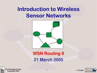
16. Routing in Sensor Networks • Large scale sensor networks will be deployed, and require richer inter-node communication • In-network storage (DCS, GHT, DIM, DIFS) • In-network processing • “Fireworks routing” • Need point-to-point routing to scale • Many nodes • Many flows • Different densities

17. Design Goals • Simple – minimum required state, assumptions • Scalable – low control overhead, small routing tables • Efficient – low routing stretch • Robust – node failure

18. GPSR: Greedy Perimeter Stateless Routing for Wireless Networks Brad Karp, H. T. Kung Harvard University

19. GPSR: Motivation • Ad-hoc routing algorithms (DSR, AODV) • Suffer from out of date state • Hard to scale • Use geographic information for routing • Assume every node knows position (x,y) • Keep a lot less state in the network • Require fewer update messages

20. GPSR Algorithm : Greedy Forwarding • Each node knows the geographic location of its neighbors and destination • Select the neighbor that is geographically closest to the destination as the next hop

21. GPSR Algorithm : Greedy Forwarding (Cont.) • Each node only needs to keep state for its neighbors • Beaconing mechanism • Provides all nodes with neighbors’ positions • Beacon contains broadcast MAC and position • To minimize costs: piggybacking

22. GPSR Algorithm : Greedy Forwarding (Cont.) • Greedy forwarding does not always work!

23. Getting Around Void • The right hand rule • When arriving at node x from node y, the next edge traversed is the next one sequentially counterclockwise about x from edge (x,y) • Traverse the exterior region in counter-clockwise edge order

24. Planarized Graphs • A graph in which no two edges cross is known as planar. • Relative Neighborhood Graph (RNG) • Gabriel Graph (GG)

25. Relative Neighborhood Graph

26. Gabriel Graph

27. Final Algorithm • Combine greedy forwarding + perimeter routing • Use greedy forwarding whenever possible • Resort to perimeter routing when greedy forwarding fails and record current location Lc • Resume greedy forwarding when we are closer to destination than Lc

28. Protocol Implementation • Support for MAC-layer feedback • Interface queue traversal • Promiscuous use of the network interface • Planarization of the graph

29. Simulation and Evaluation • 50, 112, and 200 nodes with 802.11 WaveLAN radios. • Maximum velocity of 20 m/s • 30 CBR traffic flows, originated by 22 sending nodes • Each CBR flows at 2Kbps, and uses 64-byte packets

30. Simulation and Evaluation • PacketDeliverySuccess Rate

31. Simulation and Evaluation • Routing Protocol Overhead

32. Simulation and Evaluation • Path Length

33. Simulation and Evaluation • Effect of Network Diameter

34. Simulation and Evaluation • State per Router for 200-node • GPSR node stores state for 26 nodes on average in pause time-0 • DSR nodes store state for 266 nodes on average in pause time-0

35. Pros and Cons?

36. Pros and Cons • Pros: • Low routing state and control traffic  scalable • Handles mobility • Cons: • GPS location system might not be available everywhere. • Geographic distance does not correlate well with network proximity. • Overhead in location registration and lookup • Limitations of planarization algorithm • works under unit disk model, which doesn’t hold in practical network • hard to handle mobility • planarization reduces network connectivity

37. Beacon Vector RoutingScalablePoint-to-point Routing in Wireless Sensor Networks R. Fonseca, S. Ratnasamy, D. Culler, S. Shenker, I. Stoica UC Berkeley

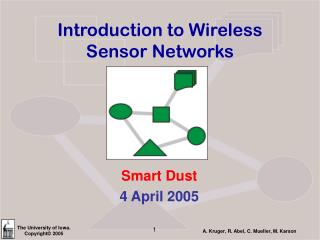
38. Beacon Vector Routing • Solution: fake geography • Create a routing gradient from connectivity information rather than geography • Nodes assigned positions based on connectivity • Greedy forwarding on this space

39. Beacon-Vector: Algorithm • 3 pieces • Deriving positions • Forwarding rules • Lookup: mapping node IDs  positions

40. Beacon-Vector: deriving positions • r beacon nodes (B0,B1,…,Br) flood the network; a node q’s position, P(q), is its distance in hops to each beacon P(q) =  B1(q), B2(q),…,Br(q)  • Node p advertises its coordinates using the k closest beacons (we call this set of beacons C(k,p)) • Nodes know their own neighbors’ positions • Nodes also know how to get to each beacon

41. Beacon-Vector: forwarding • Define the distance between two nodes P and Q as • To reach destination Q, choose neighbor to reduce distk(*,Q) • If no neighbor improves, enter Fallback mode: route towards the beacon which is closer to the destination • If Fallback fails and you reach the beacon, do a scoped flood Does the forwarding scheme guarantee reachability?

42. Beacon maintenance • Route based on the beacons the source and destination have in common • Does not require perfect beacon info. • Each entry in the beacon vector has a sequence number • Periodically updated by the corresponding beacon • Timeout • If the #beacons < r, non-beacon nodes nominate themselves as beacons

43. Location directory • Store location mapping at beacon nodes • Hashing H: nodeid → beaconid [14] • Each node k that wants to be a destination periodically publishes its coordinates to its corresponding beacon bk = H(k) • When a node wants to route to node k, it sends a lookup request to bk • Cache the coordinates

44. 0,3,3 2,1,3 3,0,3 1,2,3 3,1,2 1,3,2 2,2,2 2,3,1 3,2,1 3,3,0 Simple example B1 B2 B3

45. D=4 D=4 D=2 D=2 Fallback towards B1 D=4 D=4 D=4 D=4 Simple example Route from 3,2,1 to 1,2,3 B1 B2 0,3,3 2,1,3 3,0,3 1,2,3 3,1,2 1,3,2 2,2,2 2,3,1 3,2,1 3,3,0 B3

46. Evaluation - Simulation • Packet level simulator in C++ • Simple radio model • Circular radius, “boolean connectivity” • No loss, no contention • Larger scale, isolate algorithmic issues

47. Evaluation - Implementation • Real implementation and testing in TinyOS on mica2dot Berkeley motes • 4KB of RAM! • Judicious use of memory for neighbor tables, network buffers, etc • Low power radios • Changing and imperfect connectivity • Asymmetric links • Low correlation with distance • Two testbeds • Intel Research Berkeley, 23 motes • Soda Hall, UCB, 42 motes

48. Simulation Results

49. Effect of the number of beacons BVR, 3200 nodes Can achieve performance comparable to that using true positions

50. Scaling the number of nodesNumber of beacons needed to sustain 95% performance Beaconing overhead grows slowly with network size (less than 2% of nodes for larger networks)