Download
1 / 66
660 likes | 805 Views
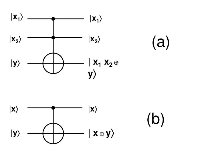
|x 1 . |x 1 . (a). |x 2 . |x 2 . | x 1 x 2 y . |y . |x . |x . (b). | x y . |y . Quantum Gates and Their Unitary Matrices. Toffoli Gate. C2NOT 3-qubit universal permutative gate The unitary operation matrix permutation matrix. Matrices of faults.

E N D
|x1 |x1 (a) |x2 |x2 | x1x2 y |y |x |x (b) | x y |y
Quantum Gates and Their Unitary Matrices. • Toffoli Gate. • C2NOT • 3-qubit universal permutative gate • The unitary operation matrix • permutation matrix
Matrices of faults. • (a) stuck-at-0 in binary quantum circuit, (b) stuck-at-1 in binary quantum circuit, (c) inverter in binary quantum circuit, (d) stuck-at-V0 in binary quantum circuit, (e) phase fault in binary quantum circuit,
ab ab 1 1 000 001 001 001 00 01 11 10 00 01 11 10 00 01 11 10 v0 v0 010 011 01V0 01V0 v1 v1 111 110 11V1 11V1 1 1 100 101 101 101 x g a (a) y r h b z s q f p c V V+ V c c c c 0 1 0 1 0 1 ab 0 1 ab 0 1 0 1 1 0 0 1 00 01 11 10 (c) (d) (e) (b)
(a) Realization of a Toffoli gate from Controlled V, Controlled V+ and Feynman gates.Places of faults are denoted by small italic letters.(b)Kmap of the fault free output f for circuit from Figure 6, and the Kmap of the same output f when there is a stuck-at-1 fault in quantum wire p, (c) symbolic output for function f for stuck-at-1 fault in wire p, (d) binary output signals of a correct circuit, (e) symbolic faulty outputs with probabilistic tests for the same fault.
ab ab 1 1 000 001 001 001 00 01 11 10 00 01 11 10 00 01 11 10 v0 v0 010 011 01V0 01V0 v1 v1 111 110 11V1 11V1 1 1 100 101 101 101 x g a (a) y r h b z s q f p c V V+ V c c c c 0 1 0 1 0 1 ab 0 1 ab 0 1 0 1 1 0 0 1 00 01 11 10 (c) (d) (e) (b)
(a) Cascading V gates creates an inverter. Measurement of intermediate state would give |0> and |1> with equal probabilities, (b) Controlled-V gate, (c) its unitary matrix, (d) Controlled-V+ gate, (e) its unitary matrix.
Input test vector Correct output vector Fault S-a-1 in p .. . .. ….. . ……... Faulty output Other outputs 000 001 010 011 100 101 111 110 000 001 010 011 100 101 110 111 001 no 011 010 101 no 110 111 1 no no 010 011 no no 111 110 1/2 1/2 1 1/2 1/2
(a) Unitary matrix of Toffoli gate, • (b) unitary matrix of Feynman gate, • (c) unitary matrix of Square-root-of-Not gate, • (d) unitary matrix of Square-root-of-Not-Hermitian gate, • (e) calculation of result on output of Square-root-of-Not gate when its input is in pure state |0>
(a) 1 0 0 0 0 0 0 0 0 1 0 0 0 0 0 0 0 0 1 0 0 0 0 0 0 0 0 1 0 0 0 0 0 0 0 0 1 0 0 0 0 0 0 0 0 1 0 0 0 0 0 0 0 0 0 1 0 0 0 0 0 0 1 0 (b) U Tof = 1 0 0 0 0 1 0 0 0 0 0 1 0 0 1 0 U Fe = (c) (d) 1+i 1-i 1-i 1+i 1-i 1+i 1+i 1-i U V = ½ U V+= ½ 1+i 1-i 1-i 1+i 1+i 1-i 1 0 = ½ = V0 U V *|0>= ½ (e)
= 0.5 0.5 = = 1+ i2 + 1 +i2 2-2i2 2-2i2 1+ i2 + 1 +i2 = = 0.25 = = = 0.25 (1+i)(1+i)+(1-i)(1-i) (1+i)(1-i)+(1-i)(1+i) (1-i)(1+i)+(1+i)(1-i) (1-i)(1-i)+(1+i)(1+i) 1+i1–i 1–i1+i 0.5+0.5i0.5–0.5i 0.5–0.5i0.5+0.5i 0.5+0.5i0.5–0.5i 0.5–0.5i0.5+0.5i 1+i1–i 1–i1+i (1+ 2i+i2)+(1-2i+i2) 2(1-i2) 2(1-i2) (1+ 2i+i2)+(1-2i+i2) = 0.25 = 1+(-1) 1-(-1) 1-(-1) 1+(-1) 0 2 2 0 0 1 1 0 1+i2 1-i2 1-i2 1+i2 1+i2 1-i2 1-i2 1+i2 = 0.5 0.5 = = = 0.5 0.5
DETERMINISTIC AND PROBABILISTIC TEST GENERATION FOR BINARY AND TERNARY QUANTUM CIRCUITS Sowmya Aligala, Sreecharani Ratakonda, Kiran Narayan, Kanagalakshmi Nagarajan, Martin Lukac, Jacob Biamonte and Marek PerkowskiPortland Quantum Logic GroupElectrical & Computer Engineering Department, Portland State University, Portland, OR 97207-0751, USA, mperkows@ee.pdx.edu
Quantum Test proposed for the first time • Quantum computing impact around year 2010. • Physical realization and synthesis of quantum circuits. • Nothing on generating tests • Nothing on fault localization • Fault models for quantum circuits not formulated. • Approach to test generation for a wide category of fault models of single and multiple faults. • Deterministic and Probabilistic tests • A Probabilistic Fault Table is created that includes probabilistic information. • Binary and ternary quantum circuits. • The system generates test sequences and adaptive trees for fault localization
Introduction • Qubit • Quantum logic gate • Unitary matrix • Binary quantum gates process qubits which can have either a |0> or |1> or both |0> and |1> at the same time to varying extents • Superposition state |0>+|> where ||2 + ||2 = 1, |x |x | x y |y
Introduction • and are complex numbers such that measurement probability of |0> is ||2 and measurement probability of |1> is ||2. • |X|2 is a result of multiplication of complex number X and its conjugate. • When the qubit state is observed or measured, it becomes invariably either |0> or |1>. Quantum world of Hilbert Space Macro world of probabilistic binary vectors |x Measurement |x 00 11 | x y 01 |y 10
1 0 0 0 0 1 0 0 0 0 0 1 0 0 1 0 U Fe = Quantum Gates and Their Unitary Matrices: Feynman. • CNOT • 2-qubit linear permutative gate
Quantum Gates and Their Unitary Matrices: Toffoli. 1 0 0 0 0 0 0 0 0 1 0 0 0 0 0 0 0 0 1 0 0 0 0 0 0 0 0 1 0 0 0 0 0 0 0 0 1 0 0 0 0 0 0 0 0 1 0 0 0 0 0 0 0 0 0 1 0 0 0 0 0 0 1 0 • CCNOT • 3-qubit universal permutative gate U Tof =
A little algebra reminder • Matrices of all quantum operations are unitary (and usually have complex numbers as entries). • Matrix X is unitary when X * X+ = I, where I is an identity matrix and X+ is a hermitian matrix of X. • Hermitian matrix of X is conjugate transpose matrix of X.
Reversibility and Permutation Matrices • Quantum gates and circuits exhibit the additional property of reversibility as their mechanism of action is through Schrödinger’s evolution (which is reversible by virtue of being unitary). • Thus, methods developed for permutative (reversible) circuits are helpful for quantum circuits as well. • Permutative circuits have only pure states and their matrices are permutative.
NOT NOT Square Root of NOT Gate • Connecting two “square root of NOT” gates in series acts as a NOT gate inverting a qubit (that is, the probabilities that the qubit will collapse to pure state |1> is changed to the probability that that the qubit will collapse to |0>, [1]). • If one measures the qubit after only one “square root of NOT” gate, the result of the measurement is unknown. |0 |1 1+i 1-i 1-i 1+i Superposition state V0 observed as random state U V = ½
Non-permutative quantum gates • This is not a permutative gate, but a truly quantum gate. • It means, applied to pure states it creates superposition states on its output. 1+i 1-i 1-i 1+i U V = ½
Step-by-step calculation of unitary matrix of an inverter gate created by multiplication of unitary matrices of Square-root-of-Not gates connected in series (standard matrix multiplication).
NOT NOT Square Root of NOT Gate Hermitian 1-i 1+i 1+i 1-i Hermitian U V+= ½ |0 |0 + Superposition state V0 observed as random state
Controlled gates a P 1 0 0 0 0 1 0 0 0 0 1+i 1-i 0 0 1-i 1+i 1/2 b Q V a P 1 0 0 0 0 1 0 0 0 0 1-i 1+i 0 0 1+i 1-i 1/2 b Q V+
All Possible States • Let us now try to find, by matrix/vector multiplication, all possible states that can be created by applying all possible serial combinations of gates V and V+ to states |0> , |1> and all states created from these pure states • A qubit |0> given to a “square root of NOT” gate gives a state denoted by |V0>. • After measurement this state gives |0> and |1> with equal probabilities ½. 1+i 1-i 1-i 1+i 1+i 1-i 1 0 = ½ = V0 U V *|0>= ½
Calculating all possible superposition states that can be obtained from pure states |0> and |1> using V and V+ gates.
When the qutrit state is observed or measured, it becomes either |0>, |1> or |2>. • Quantum gates and circuits exhibit the additional property of reversibility as their mechanism of action is through Schrödinger’s evolution (which is reversible by virtue of being unitary). • Thus, methods developed for permutative (reversible) circuits [12,15] are helpful for quantum circuits as well. • Permutative circuits have only pure states and their matrices are permutative [11].
Introduction • Qubit • Quantum logic gate • Unitary matrix • Binary quantum gates process qubits which can have either a |0> or |1> or both |0> and |1> at the same time to varying extents and hence exhibit a superposition state |0>+|> where ||2 + ||2 = 1, • and are complex numbers such that measurement probability of |0> is ||2 and measurement probability of |1> is ||2. • |X|2 is a result of multiplication of complex number X and its conjugate. When the qubit state is observed or measured, it becomes invariably either |0> or |1>. • Ternary quantum gates process qutrits which can be pure state |0>, |1> or |2> or any combination of |0>, [1> and |2>, a superposition state |0> + |> + |> where ||2 + ||2 + ||2 = 1, , and are complex numbers such that measurement probability of |0> is ||2, measurement probability of |1> is ||2 and measurement probability of |2> is ||2, [10,11].
As we see, after obtaining states |0>, |1> |V0> and |V1> the system is closed and no more states are generated. • Therefore the subset of (complex, continuous) quantum space of states is restricted with these gates to a set of states that can be described by a four-valued algebra with states { |0>, |1>, |V0>, |V1> }. • We assume here for simplification of explanation that only faults s-a-0, s-a-1, s-a- V0, and s-a-V1 are possible, but many other fault models can be defined.
The Test Generation Problem • Find a sequence of input vectors (tests) that applied to the circuit will either confirm that the circuit is correct or will determine that it has one or more faults from certain library of faults. • single-fault model • multiple-fault model • The reversibility property notably simplifies the problem of testing reversible circuits compared to irreversible circuits • Basic quantum gates: • Toffoli, • Feynman, • CV (controlled square root of NOT) • CV+ (controlled square root of NOT Hermitian gate). • arbitrary (binary or ternary) quantum gates • broad fault models • stuck-at pure states, • stuck-at superposition states, • bridging-AND, • bridging-OR, • shift of value, • phase shift, • gate change • and many others
Matrices of faults. Fault Models used in the Algorithm. • Fault matrices • square, • complex, • non-unitary • Unitary • Not only stuck-at fault matrices. • The matrices of stuck-at faults are not unitary, but some other fault matrices may be unitary • changing phase • inserting a Pauli rotation.
1 0 1 0 0 1 0 1 0 1 1 0 1+i 1-i 1+i 1-i 1 0 0 i (c) (e) (a) (b) stuck-at-0 in binary quantum circuit, stuck-at-1 in binary quantum circuit, inverter in binary quantum circuit 1 stuck-at-V0 in binary quantum circuit, 2 phase fault in binary quantum circuit Matrices of faults.
Matrices of faults stuck-at-entangled-state-01-10 of two quantum wires. 1 0 0 0 1 0 0 0 1 0 0 0 0 0 0 1 0 1 1 0 0 1 1 0 0 1 1 0 0 1 1 0 0 0 1 0 0 1 0 0 1 0 1 0 0 0 1 0 0 1 stuck-at-2 in ternary quantum circuit, (f) (g) (h) truncated plus 1 in ternary quantum circuit AND-bridging fault in binary quantum circuit
Fault Models used in the Algorithm. • The fault model in our system is that a fault matrix is inserted in place of the fault, more formally, the fault matrix is inserted in the netlist of parallel-serial connections of unitary matrices of gates.
Principles of Test Generation for Binary Quantum Circuts • A quantum equivalent of stuck-at faults. • Gate is stuck to a pure state or a superposition state • If the circuit contains only permutative gates and (controlled by pure signals) gates V and V+, the four values listed above; { |0>, |1>, |V0>, |V1> } can occur as the correct and the stuck-at values. • We call it “four-valued algebra” keeping in mind that V0 and V1 are symbolic representations of pairs of real numbers, as shown earlier. First a simplified model.
In general, symbols correspond to groups of complex numbers. • The output measurements of a faulty circuit is in general probabilistic, because of the use of the non-permutative quantum gates such as Controlled-V, resulting in measured random outputs. • By comparing the faulty output (in general, a vector of complex numbers) with the faultless output (a binary vector), it can be observed whether the test for this fault is deterministic or probabilistic.
Simple Example: Testing the quantum realization of the Toffoli gate x g a y r h b f z s q p c V V+ V Every quantum wire, denoted by a letter x, y, z, p, r, q, s can be stuck to one of the values: { |0>, |1>, |V0>, |V1> }.
x g a y r h b z s q f p c V V+ V 1 1 0001 11 10 v0v0 v1 v1 1 1 symbolic output for function f for stuck-at-1 fault in wire p Kmap of the same output f when there is a stuck-at-1 fault in quantum wire p Kmap of the fault free output f for circuit c c 01 0 1 ab ab 0 1 0 1 1 0 0 1 00 01 11 10 000 is a deterministic test 011 is a probabilistic test
probabilistic tests versus deterministic tests • The internal signals (complex numbers) of the quantum world cannot be observed by the testing program. • Only the externally measured classical signals |0>, |1> (for binary) or |0>, |1>, |2> (for ternary) in the classical world are observed and measured at the input to the Tester Program. • We know, however, from the symbolic output what binary vector values can occur and with what probabilities on the output. • So all possible measurement vectors can be known in advance with their probabilities. • If these values can collapse to the correct output vector (of a non-faulty circuit) they are called probabilistic tests, otherwise they are called the deterministic tests. • If they are the same in the faulty and non-faulty circuit then they cannot be used as tests for this fault which is represented by a zero or a blank cell in the Fault Table.
x g a y r h b z s q f p c V V+ V ab ab 001 001 000 001 00 01 11 10 00 01 11 10 01V0 01V0 010 011 111 110 11V1 11V1 100 101 101 101 Kmap of the same output f when there is a stuck-at-1 fault in quantum wire p Kmap of the fault free output vector for circuit c c symbolic faulty outputs with probabilistic tests for the same fault. 0 1 0 1
Selecting deterministic and probabilistic tests to test and fault localization sequences • If the outputs are “deterministic”, we apply test vectors and detect the fault using standard deterministic approach to testing. • If the outputs are “probabilistic” (complex numbers denoted by symbolic values like V0 and V1 in our case), we calculate the probability of occurrence of the observed output as explained in the following sections. • We give priority to deterministic tests. • Observe that a deterministic fault in quantum circuit can be observed on the output probabilistically. • There are also probabilistic faults that are observed probabilistically.
Probability calculation of the random output • By iteratively applying the same input test vector (a probabilistic test) we are calculating the probability of getting the observed output. • The input vectors are always vectors of pure states. • Each successive iteration reduces the probability of obtaining a correct measurement for a faulty circuit. For five iterations the probability of obtaining a correct measurement in presence of a given fault is reduced to 1/32. • Similarly for six iterations it is 1/64 and for eight iterations it is 1/256 (See Figure 8). • Hence, the greater the number of iterations the lesser is the probability of getting the correct measurement for faulty circuit. • Suppose that we use test 110 for fault S-a-1 in location p. • According to Fig. 7d the correct output should be 111 and according to Figure 7e the faulty output is 11V1, which means 110 or 111 with equal probabilities of ½ are measured. • If we tested eight times and we get |1> in bit f each time, we have the probability 255/256 that there no fault S-a-1 in location p. • Of course, in this particular case we should apply deterministic tests a’b’c’ or ab’c’ since they are possible. In general, probabilistic tests may not exist. The number of iterations should depend on the expected accuracy and cost of testing.
Probabilistic Supernode – a tree for calculating the probability of obtaining a sequence of n signals “1” from a gate which has probability ½ of output “1”.
From binary to ternary logic • PROPOSITION 1: Under the single stuck-at-fault model (i.e. stuck-at-0 and stuck-at-1 in binary), a test set is complete if and only if each of the wires at every level can be set to |0>, |1> and |2> by the test set. • PROPOSITION 2: Any test set that is complete for the single stuck-at-fault model is also complete for the multiple stuck-at-fault model. • LEMMA 1: Each test vector covers exactly two-third of the faults, and every fault is covered by exactly two-thirds of the possible test vectors. • It is straightforward to further generalize these results to a multiple-valued logic with arbitrary radix. • Thus similar propositions and lemma can be used in quantum or reversible logic of any radix.
Testing the ternary reversible circuit • The gates are ternary Feynman gates, they use modulo 3 addition instead of EXOR (which is a modulo 2 addition). • The analogy to binary case is straightforward.
Because in reversible logic there are relatively many tests for each fault, the test generation is easier than in irreversible logic. • Creating fault tables and adaptive trees for fault localization for binary and ternary reversible logic and quantum computing is very similar.
Test Generation and Fault Localization System • . • The system for test generation and fault localization in binary and ternary quantum circuits is shown in Figure 10. We generate tests and use them to localize the fault in quantum circuits (details about fault localization are in [15]). Localization is done using an adaptive tree (decision tree, diagnostic tree, fault tree). In adaptive tree there are two types of nodes, deterministic nodes which are the same as in standard decision (adaptive) tree, and probabilistic supernodes (which represent small trees of probabilistic tests like one from Figure 8). In contrast to reversible circuits [15] where forward and backward fault simulation is applied for the test generation efficiency, in case of quantum circuits only forward simulation is possible since using backward simulation from the arbitrary fault point back to inputs may result in mixed (superposition) states on inputs, and we can create only pure states on the circuit inputs. The algorithm for quantum fault simulation is similar to standard fault simulation in a irreversible circuit, only the fault model is more general now. • The sequence of steps is as follows. • 1. Preprocessing the netlist. • First the circuit is preprocessed to a form for which it is possible to apply operators of Kronecker multiplication (for parallel connection of sub-circuits (gates, blocks, columns). Standard matrix multiplication are applied for serial connection of gates (columns). As seen in Fig.12, swap gates are introduced in such a way that the circuit is build from parallel and serial connections of blocks. This allows to calculate a resultant matrix of each column using Kronecker multiplications. This was not possible if a wire was crossing a gate description as in Figure 12a in the first gate from the left. • 2. Creating a resultant unitary matrix of a correct circuit.
A non-faulty circuit is simulated for all pure state input combinations to create a fault-free table like that from Figure 7d. It is done as follows. The program calculates the resultant transition matrix of the correct circuit from component matrices of gates (unitary) and faults (usually non-unitary). Operations of Kronecker matrix multiplication and standard matrix multiplication are used to calculate the resultant matrices of non-faulty and faulty circuits [10]. • 3. Calculation of all correct output vectors corresponding to input vectors. • The resultant matrix of the correct circuit is multiplied by the vector of all possible (pure state) input vectors to obtain the vector of all corresponding output vectors.
4. Generating tests for every possible fault • Every single fault is inserted and all tests for it are generated as in Figure 7e (currently we use exhaustive methods as in points 2,3 above). • Assume a fault F1 is inserted in place X. It means, a value different than the stuck-at value should be in this place. (If a correct value is V0 then 0, 1 and V1 are faulty values in our case). • This way, for certain input vector, a vector of faulty values is created in the place and level of the fault. • Every fault is simulated by inserting a unitary or non-unitary transition matrix in the location of this fault. • For stuck-at faults the matrices are non-unitary.