Download
1 / 1
10 likes | 81 Views
Control of a free-surface barotropic model of the Bay of Biscay by assimilation of sea-level data in presence of atmospheric forcing errors. J. Lamouroux (1) (lamourou@notos.cst.cnes.fr) , P. De Mey (1) , F. Lyard (1) , F. Ponchaut (2) , E. Jeansou (2).

E N D
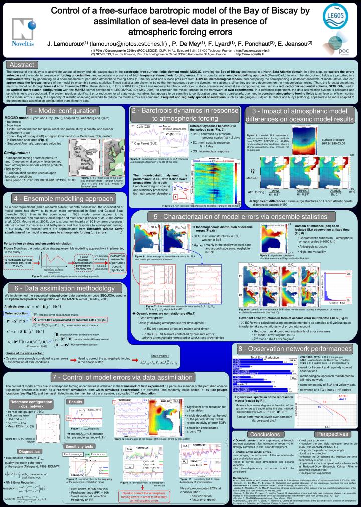
Control of a free-surface barotropic model of the Bay of Biscay by assimilation of sea-level data in presence of atmospheric forcing errors J. Lamouroux(1) (lamourou@notos.cst.cnes.fr) , P. De Mey(1), F. Lyard(1), F. Ponchaut(2), E. Jeansou(2) (1) Pôle d’Océanographie Côtière (POC-LEGOS), OMP, 14 Av. Edouard Belin, 31 400 Toulouse, France : http://poc.omp.obs-mip.fr (2) NOVELTIS, 2 av. de l’Europe, Parc Technologique du Canal, 31526 Ramonville St Agne, France : http://www.noveltis.fr Abstract The purpose of this study is to assimilate various altimetry and tide-gauges data in the barotropic, free-surface, finite element model MOG2D, covering the Bay of Biscay and nested in a North East Atlantic domain. In a first step, we explore the errors sub-space of the model in presence of forcing uncertainties, and especially in presence of high frequency atmospheric forcing errors. This is done by an ensemble modelling approach (Monte-Carlo) in which the atmospheric fields are perturbed in a multivariate way : by generating an a priori ensemble of perturbed atmospheric forcing fields (10 meters wind and surface pressure from ARPEGE meteorological model), and computing the corresponding a posteriori ensemble of model states, one can approximate the forecast errors of the model by ensemble spread statistics. These statistics are shown to be neither homogeneous over the domain, nor stationary, since they are very dependent on the meteorological forcing. Then, the forecast covariance matrix is modelized through forecast error Ensemble EOFs. These statistics, in form of 6D-EOFs (Sea Level Anomaly, barotropic velocities, surface pressure and wind-stress components), are used in a reduced-order sequential scheme, SEQUOIA, used in an Optimal Interpolation configuration with the MANTA kernel developed at LEGOS/POC (De Mey, 2005), to constrain the model forecast in the framework of twin experiments. In a reference experiment, the data assimilation system is calibrated and sensitivity tests are conducted. The system provides significant error reduction for all state vector variables, but appears to be sensitive to configuration parameters : particularly, one need to constrain atmospheric forcing fields to achieve an efficient control of the model errors. Finally, the capability of realistic observing networks to reduce the model errors are compared. Frequent and regularly spaced observations, such as tide-gauges (SLA) or HF radars and buoys (velocity), appeared to be more adapted to the present data assimilation configuration than altimetry data. (MOG2D) 2 - Barotropic dynamics in response to atmospheric forcing 1 - Model configuration 3 - Impact of atmospheric model differences on oceanic model results MOG2D model(Lynch and Gray (1979), adapted by Greenberg and Lyard) • barotropic • Non linear • Finite Element method for spatial resolution (refine study in coastal and steeper • bathymetry area) • zone = Bay of Biscay (BoB) + English Channel (EC) + Celtic Sea (CS), nested • in European shelf area (Fig. 1) • Sea Level Anomaly, barotropic velocities Different dynamics behaviour in the various seas (Fig. 2) : Cork (CS) Wight (EC) • BoB : controlled by pressure • temporal scales (ts) ~ 2 days • EC : non-isostatic response • ts ~ 1 day • CS : intermediate response Figure 4 : model SLA response to various atmospheric forcing products from ECMWF, ARPEGE and ALADIN models (down) at a fixed time, where a strong atmospheric low crosses the domain (up) Cap Ferret (BoB) Celtic Sea (CS) EC Figure. 2 : comparison of model and IB SLA response to atmospheric forcing in 3 points of the area Bay of Biscay (BoB) surface pressure 26/12/1999 03:00 Configuration : Model • Atmospheric forcing : surface pressure • and 10 meters-wind velocity fields derived • from atmospheric models ARPEGE products. • Tide forcing • European shelf solution used as open • boundary conditions • Time period : 16/11/1999, 00:0001/12/1999, 00:00 Inverse Barometer The non-isostatic dynamic is predominant in EC, with Kelvin wave propagation (along both French and English coasts) and stationary processes; it’s much weaker elsewhere. 60 Figure. 1 : FE mesh used in the study: Bay of Biscay (BoB) + English Channel (EC) + Celtic Sea (CS) nested in European shelf 4 - Ensemble modelling approach 2 coeffs Significant differences : storm surge structures on French Atlantic coasts, differences patches in EC Ensemble methodology Figure. 3 : Non-isostatic response along sections 1 and 2 of the domain 1 t a0 a1 a2 a3 -15 ARPEGE 6h, 0.25° ALADIN 3h, 0.1° Combining and time interpolation ECMWF 6h, 0.5° (cm) Atm. forcing : 5 - Characterization of model errors via ensemble statistics +1 Domain of influence (doi) of an isolated SLA observation at fixed time (Fig.8) : • Inhomogeneous distribution of oceanic errors (Fig.6) : • SLA : max. error structures in EC, • weaker in BoB • Ubt, Vbt : mainly in the shallow coastal band • and around cape zone, negligible • in BoB • Characteristic dimension ~ atmospheric • synoptic scales (~1000 km) • Anisotropic structure • High time variability Perturbation strategy and ensemble simulation: Figure 5 outlines the perturbation strategy/ensemble modelling approach we implemented in the study : +0.5 As a prior requirement (and a research subject) for data assimilation, the specification of model errors has shown to be much more complicated in Shelf and Coastal Seas (hereafter SCS) than in the open ocean : SCS model errors appear to be inhomogeneous, non-stationary, anisotropic and multi-scale (Echevin et al., 2000; Auclair et al., 2003; Mourre et al., 2004), due to strong non-linearity of SCS dynamic processes, intense control of coastlines and bathymetry, and fast response to atmospheric forcing. In our study, the forecast errors are approximated from Ensemble (Monte Carlo) simulations of the model in response to atmospheric forcing (p, ) errors. Figure 8 : significant correlation of a SLA measure at Weymouth with SLA field Figure 6 : time average of ensemble variance for SLA and barotropic current components SLA |Ubt,Vbt| A Figure 5 : perturbation strategy/ensemble modelling approach B 6 - Data assimilation methodology We implemented the sequential reduced-order data assimilation code SEQUOIA, used in an Optimal Interpolation configuration with the MANTA kernel (De Mey, 2005). Analysis step : Explained variance (%) Order reduction Figure 9 : oceanic error multivariate EOFs (first two dominant modes) and spectrum of variance explained by each mode (the first 20) Oceanic errors are non-stationary (Fig.7) #1 • ~24h error growth • closely following atmospheric error development : Covariant error structures in form of oceanic error multivariate EOFs (Fig.9) a posteriori ensemble of perturbed oceanic trajectories 300 MOG2D simulations 100 EOFs were calculated using ensemble members as samples at 5 various dates in order to take non-stationarity of errors into account A priori ensemble : 300 atmospheric perturbations Pp, Uwp, Vwp Modes (120) 10 multivariate EOF(t,X) of reference atm. fields P, Uw, Vw - In EC (A) : oceanic errors are mainly wind-driven • Red spectrum good representativity of error structures • 1st mode : error “regime” in EC • 2nd mode : shelf error “regime” run on a Linux cluster #2 • In BoB (B) : SLA errors controlled by pressure errors; • velocity errors partially correlated to wind-stress uncertainties Figure 7 : time evolution of ensemble variance for SLA, Ubt, Vbt, IB SLA, , at points A and B (Pham et al., 1998) 8 - Observation network performances choice of the state vector : State vector : 4TG, 10TG, 21TG : 4,10,21 tide-gauges 4ALT : Jason+Topex+GFO+Envisat – 15 days 4R2B : 4 HF radars sites + 2 anchored buoys • Oceanic error strongly correlated to atm. errors • Fast evolution of atm. conditions Need to correct the atmospheric forcing in the analysis step Total Error Reduction • need for frequent and regularly spaced • observations • methodological approach maladapted to • altimetry network • complementarity of SLA and velocity data • relevance of a TG + buoy + HF radars : forecast error covariances matrix 7 - Control of model errors via data assimilation : error EOFs approximated by ensemble EOFs (cf. §5) : error variances of mode k The control of model errors due to atmospheric forcing uncertainties is achieved in the framework of twin experiment : a particular member of the perturbed oceanic trajectories ensemble is taken as a “control” simulation, from which simulated observations are extracted (and randomly noise added) at 10 tide-gauges locations (see Fig.10), and then assimilated in another member of the ensemble, a so-called “free” simulation. : observation error covariances matrix Eigenvalues spectrum of the representer matrix (scaled by R) : : reduced-order (RO) representer Reference configuration / obs. network Results : RO observation operator Measure how many degrees of freedom of the system errors are captured by the obs. network (independently of DA) • Significant error reduction for • all variables • visible degradation at the end • of the period (storm) : weak • representativity of error EOFs • correction zone located • around TG 10TG mean = 0.46 • 10 real tide gauges (10TG) • 1.5 cm rmserror • Obs : • Mean EOFs (cf. §5) 4ALT 18 Similar performance levels over dominant (large-scale) d.o.f. 0.5 RMSRE(XY) RMSRE(t) 15 1 Eigenvalues Figure 11 : Jmin diagnostic Perspectives Conclusions mean(Jmin)~0.5 ensured for ensemble variance=1/3 Figure 10 : 10 TG reference network Figure 12 : diagnostics of the control of the model errors by the system • Oceanic errors : inhomogeneous, anisotropic and non-stationary ; fast evolution of errors (~24h) strongly correlated to atm. error development. • Control of the model errors : • encouraging performances of the reduced-order data assimilation system • need to correct both atmospheric and oceanic variables • the time-dependency of errors should be considered • real data experiment • consider the atm. field resolution error in our study (with ALADIN, AROME f.i.) • improve the prediction range length : • localize the correction • enhance the OI scheme (f.i. improve the time-dependency of error EOFs) • implement a more complex/costly scheme such as Reduced-Order Ensemble Kalman Filter or Ensemble Kalman Filter • multiple twin-experiment d.o.f. RERMS(XY) Sensitivity tests SLA RERMS(XY) SLA Diagnostics days • cost function minimum : • qualify the intern coherency • of the system (Talagrand, 1999, ECMWF) Prediction range Pure forecast Ubt mean EOFs 6h 12h 24h Ubt with p the number of assimilated obs. RERMS(XY) References Figure 13 : sensitivity test to the frequency of the correction – Prediction range Figure 15 : sensitivity test to time-dependency of error statistics • Lynch, D.R. and Gray, W.G. A wave equation model for finite element tidal computations. Computers and Fluids, 7:207-228, 1979 • Echevin, V., De Mey, P., Evensen, G. Horizontal and vertical structures of the representer functions for sea surface measurements in a coastal circulation model. J. Phys. Oceanog., 30:2627-2635, 2000 • Auclair, F., Marsaleix, P., De Mey, P. Space-time structure and dynamics of the forecast error in a coastal circulation model of the Gulf of Lions. Dyn. Atm. Oceans, 36:309-346, 2003 • Mourre, B., De Mey, P., Lyard, F., and Le Provost, C. Assimilation of sea level data over continental shelves : an ensemble method for the exploration of model errors due to uncertainties in bathymetry. Dyn. Atm. Oceans, 38:93-121, 2004 • De Mey, P., The MANTA analysis kernel, Pers. Comm., 2005 • Lamouroux, J., De Mey, P., Lyard, F., Jeansou, E. Control of a barotropic model of the Bay of Biscay in presence of atmospheric forcing errors. Submitted to J. Geophys. Research-Oceans, 2006 • RMS Error Reduction : Figure 14 : sensitivity test to atmospheric correction Use of pre-computed EOFs at analysis time : RMSER(XY) : • Best control for 6h-analysis • Prediction range (PR) ~ 30h • Small impact of correction • frequency on PR Need to correct the atmospheric forcing errors in order to efficiently control oceanic errors • best correction • faster error growth RMSER(t) :