Download
1 / 33
390 likes | 769 Views
Net Present Value (NPV), Internal Rate of Return (IRR) and Modified IRR (MIRR). Lonnie Chrisman, Ph.D. Lumina Decision Systems Analytica User Group Part 1 : 20 Nov 2008 Part 2: 4 Dec 2008. Uses NPV and IRR. Capital budget planning, e.g. Choosing between investments

E N D
Net Present Value (NPV),Internal Rate of Return (IRR)and Modified IRR (MIRR) Lonnie Chrisman, Ph.D.Lumina Decision SystemsAnalytica User GroupPart 1 : 20 Nov 2008 Part 2: 4 Dec 2008
Uses NPV and IRR • Capital budget planning, e.g. • Choosing between investments • Deciding whether to fund new projects • NPV and IRR are metrics used to compare the valuation of alternative cash flows over time.
Present Value Question: Which is worth more? $10,000 to be received with certainty one year from today, or: • $10,000 received right now? • $9,500 received now? • $9,000 received now? • $8,000 received now? Estimated present value: __________
Factors influencing time-value of money • Inflation. • Risk-free rate of return. • Opportunities to put money to work. • Alternative investments. • Your remaining lifespan. • Financing rate. • Uncertainty (?)
Discount Rate • Quantifies your time-value of money, as a % per time-period (often %/year). • Exercise 1: Using your present value of $10,000 received in one year, compute your implied discount rate. If you felt $10,000 in one year is worth $9,300 now, your discount rate would be: r = 10000/9300 – 1 = 7.5%
Present Value Exercises Exercise 2: Using a discount rate of 10%/yr, what is the present value of $10,000 received in: • 2 years? • 10 years? • 6 months? • 3 months?
Cash Flow & NPV Exercise 3: A $10,000 investment (a possible project) will return $2,000 annually for 10 years. • Represent this cash flow in Analytica. • (There are 11 cash flow “events”) Using a 12% discount rate: • Compute the present value (in Analytica) of each cache flow event. • Compute the net present value for this investment. • Should you make the investment?
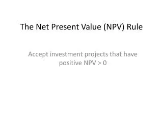
Interpreting NPV Assuming perfect cash-flow knowledge: • NPV > 0 Investment adds value. Proceed with project. • NPV < 0 Reject project • Projects (investments) are often mututally exclusive. Pursue option with max(NPV) as long as its NPV>0. • NPV = maximum you are willing to pay today to guarantee the future cash flow. • But… NPV is only one consideration. Organizations also have non-monetary objectives to consider.
NPV function’s offset • The NPV (in both Analytica and Excel) assumes the first point is 1 time period in the future. Present value is: • NPV(r,cashFlow,T) * (1+r) or • cashFlow0 + NPV(r,cashFlow,futureT)
NPV Exercises Exercise 4: A real estate investment of $200K will result in monthly rental earnings of $1K for 8 years, and will then be sold (with certainty) for $250K. • Compute the NPV for this investment. • Assume annual discount rate = 8% • Graph the NPV-curve for all discount rates from 0% to 20%. • Compare NPV-curve if you increase rental earnings 2% each year.
More NPV exercises Exercise 5: A $1.5B nuclear power plant with a 30 year lifetime will generate $200M per year for 30 years (realized at the end of each year), and then cost $5B to decommission on the 31st year. • Compute the NPV using an 8% discount rate. • Graph the NPV for discount rates ranging from 0% to 20%.
XNPV – unequal time periods Exercise 6: • A $100K investment on 4 Dec 2008 pays a $2K dividend on 1 Jan 2009, another on 1 June 2009, and then returns your $100K on 1 Aug 2009. • Using discount rate = 10%, use XNPV to compute the net present value.
Investment Decisions using NPV Exercise 7: A $10,000 treasury note with 3.5% coupon rate, matures on 15 Dec 2009. If you require a 2% return, how much are you willing to pay on 4 Dec 2008? Actual quote (4 Dec 2008): $10,459.06Should you buy it?
Uncertain Cash Flows (ENPV) A proposed product: • Requires Poisson(9) months to develop, • at LogNormal(µ:10K,σ:3K) per month. • Will launch if successful, P(success)=60% • After launch, monthly earnings for Poisson(24) months: • Earningsm~Normal(10K,8K) Exercise 8: (use monthly discount_rate=1%) • Build a model of this cash flow. • Graph: Bands(cash_flow) • Compute NPV. • Compute: E[NPV], Graph: PDF(NPV)
Interpreting NPV with Uncertainty • What is the criteria for pursuing a project/investment? • ENPV>0? • getFract(NPV,10%)>0? • ENPV>0 and getFract(NPV,1%)>-100K? • Expected return / risk tolerance tradeoff…
Net Present Utility Motivations: • Incorporating risk-tolerance or risk-adversity. • Non-monetary considerations, e.g.: • Community good will • Economic development • Strategic fit • Staff skill development • U(earnings,cgw,ed,sf,skd) – utility is a non-linear function of earnings and other factors. • NPV(r,U,T) – can be used to compute and base decisions on NPU. • When U captures risk-tolerance, ENPV>0 serves as a go/no-go decision criteria.
Obtaining Corporate Discount Rate from Stock Price • From Capital Asset Pricing Model (CAPM) Parameters: • d = corporate discount rate (rate shareholders expect from investments). • β = stock price “beta”=Cov(stock,market)/Var(market) • rf = Risk-free rate of interest • E[Rm] = Expected return from the stock market.
CAPM Exercise Exercise 9: Find the shareholder-implied discount rate for AAPL, using β=1.93, E[Rm]=8% (ave. return from NASDAQ 1980-2008), rf=1.5%.
Rate of Return • Exercise 10: A $10,000 investment today pays $15,000 in 3 years. What is the annual rate of return?
Internal Rate of Return (IRR) Exercise 11: A $1M investment returns $200K per year for 10 years. What is the rate of return? • Plot the NPV of this investment as a function of discount rate (from 0-20%) • Use IRR function to find rate or return. • Compare to an annual return of $180K or $220K per year. • Graph IRR as annual return varies from $100K to $300K.
IRR in perspective • IRR measures the quality or efficiency of an investment, but not the magnitude. • Has intuitive appeal, extremely widely used in practice. • Does not require a discount rate. • Many downsides – can be extremely misleading. Highly non-robust. • Shunned by textbooks and academics. Prevailing wisdom: Use NPV, avoid IRR!
IRR has many downsides • Exercise 12: Return to NPV graph for our nuclear power plant in Exercise 5 ($1.5B initial cost, $5B decommission cost at 30y, $200M earnings per year). • What is the rate of return for this project?
IRR is not uniquely determined • IRR may have multiple solutions: • Up to as many solutions as there are sign changes in the cash flow. • IRR may also have zero solutions: • E.g., Zero sign changes. • Common example: Project never reaches profitability.
IRR can mislead Contradictory results when costs come after revenue. Lower IRR can be better. • Exercise 13: Graph the NPV-curve (0-10%) for these two cash flows, and compute IRR:
IRR distorts apparent value of intermediate returns • Appears as if your positive intermediate earnings can be re-invested at IRR rate. • Makes options with exceptionally high IRR look too good. • Appears as if your negative intermediate expenses are financed from the start at IRR rate. • Makes bad projects look too good, good projects with late cash flow look bad. In practice, these distortions are often huge, and highly relevant – compensating for them drastically changes relative merits. Note: MIRR helps here (discussed later).
IRR and UncertaintyExpected Rate of Return • E[IRR] is non-sense! • Is usually does not exist. (e.g., non-zero probability that project never turns profit). • Will usually be NaN in a Monte-Carlo simulation • When it does exist, its results don’t make sense. • Median may exist when Mean doesn’t, but is also nonsense. • Exercise 14: A $1000 investment returns $1100 with 50% or $900 with 50% after T years. Compute the EIRR for T=[0.5, 1, 2, 4] years. • Note: The expected rate of return is “obviously” 0% in all four cases, right? What is the EIRR?
Expected Rate of Return • “Expected rate of return” more accurately describes the discount rate where the ENPV-curve crosses zero. • This is not the same as E[Irr(v,T)]! • It is equal to Irr(E[v],T) • Technically called “IRR of the Expected Cash Flow”. • Behaves more intuitively as expected. • Still suffers from same drawbacks as IRR with certain cash flows, of course.
Exercise: Expected Rate of Return A proposed product (from Exercise 8): • Requires Poisson(9) months to develop, • at LogNormal(µ:10K,σ:3K) per month. • Will launch if successful, P(success)=70% • After launch, monthly earnings: • Earningsm~Normal(10K,8K) • Exercise 15: • Compute Irr of expected cash flow. • Compare to graph computed during NPV section. • Attempt to compute E[Irr]. Does it work?
Modified IRR (MIRR) • MIRR is a variation of NPV that expressed as a rate-of-return. • Robustness of NPV • Intuitive appeal of IRR • Avoids IRR distortions • Requires: • reinvestRate (rrate): Interest rate we can expect to receive on positive flows. • financeRate (frate): Interest rate we expect to pay to finance negative flows.
MIRR details Idea: (index T := 0..n) • All positive flows are re-invested at rrate until project end (Time=Tn). • PV equivalent to all gains arriving on Tn. • gain := Npv(rrate,posFlows,T) * (1+rrate)n+1 • All negative flows financed at frate is equivalent to all expenses occurring at T0 (index T:=0..n) • cost := Npv(frate,negFlows,T)*(1+frate) • MIRR = (gain/-cost)1/n-1
MIRR Exercises Exercise 16: • Create a User-Defined Function to compute MIRR. Exercise 17: • Compute the MIRR for these cash flows from the earlier “IRR can mislead” exercise using rrate=frate=6%.
Summary • It matters when a cash flow occurs. “Time value of money”. • Discount_rate quantifies our own time-value of money. • Inflation, risk-free investment, other opportunities, remaining lifespan, financing rate, etc. • NPV captures the magnitude of a return. • IRR and MIRR capture the efficiency (quality) of an investment. • IRR is heavily used in practice, but often highly misleading. Its upside is that it does not require any discount rate estimates. • The Monte-Carlo simulation of IRR is nonsense. IRR is poorly suited for uncertain cash flows. • NPV and MIRR are robust and meaningful when used with Monte-Carlo simulation.