Download
1 / 19
190 likes | 319 Views
Image Modeling & Segmentation. Aly Farag and Asem Ali Lecture #4-6. Image Modeling. Intensity. Spatial. Image Segmentation. Interaction. Image. Shape. Others. I NTRODUCTION. Random Field Graphical Models Representation Bayesian Network Markov Random Field Markov System

E N D
Image Modeling & Segmentation AlyFarag and Asem Ali Lecture #4-6
Image Modeling Intensity Spatial Image Segmentation Interaction Image Shape Others
INTRODUCTION • Random Field • Graphical Models Representation • Bayesian Network • Markov Random Field • Markov System • Markov process • Markov Chain • Hidden Markov Models • Tutorials by Andrew W. Moore professor of Robotics and Computer Science at CMUhttp://www.autonlab.org/tutorials/ • “Markov Random Field: Theory and Application” Class notes by Kyomin Jung, Ph.D. fromMIT Mathematics department. http://web.kaist.ac.kr/~kyomin/Fall09MRF/ • “Markov-Gibbs Random Fields in Image Analysis and Synthesis: A Review” Technical Report by Asem Ali • “A Tutorial on Hidden Markov Models and Selected Applications in Speech Recognition”, by LAWRENCE R. RABINER
Computing a Joint Probability ( Bayes Rule) Bayes, Thomas (1763) An essay towards solving a problem in the doctrine of chances. Philosophical Transactions of the Royal Society of London, 53:370-418
N f g 1 = 2 f g f f f g g g P n f 6 2 b h 2 P N P N N N N i N t t ; ; p p ; 2 : : : p p q p q 2 s z a p c y e q n x q = = = q r p q p ; ; ; ; ; ; ; ; ; Problem Formulation & Spatial Interaction Image has a natural structure in which pixels are arranged in 2D array. set of image pixel Neighborhood system in is the set of all neighboring pairs Example up to the 5th order 1st order neighborhood system 5 4 3 4 5 a z 4 2 1 2 4 b p q x t 3 1 p 1 3 c y s r 4 2 1 2 4 3 x 5 image 5 4 3 4 5 The neighborhood system satisfies a) b)
n F f f g f g 3 6 f g g L P F f f f f f f f I I F G F I G K Q L P K I F I F K Q I = 2 2 1 0 2 1 1 f g L P : : = = = = = ! ! ¡ 1 1 1 2 2 2 n n n ; ; ; ; ; ; ; : ; ; : : : : : ; : : : : : ; : : ; : ; ; : ; Problem Formulation & Spatial Interaction Observed Image Labeled Image set of gray levels (e.g., =256 in 8-bit gray image) set of labels. # classes (e.g., ) observed image. labeled image. set of all labelings (e.g., in this case different labeling sets) set of random variables defined on , and is a configuration of the field
( ( ) ( ) ) f f f f l l f F F F P N P P 1 0 > F o r a 2 = = . , ( j ) ( j ) f f f f P F F P F F 2 p p g = = = = = f g f N N P P ¡ ¡ p p p p . , p p ( j ) f f h f l l P F F i i 3 t t s e s a m e o r a s e s p = = N N p p . , p p Problem Formulation & Spatial Interaction is a Markov Random Field (MRF) w.r.t if its probability mass function abbreviated by satisfies Positivity MarkovProperty Homogeneity a Markov property establishes the local model b ? q c
1 X ¡ ( ) ( ( ) = ) C V Z T f f P T Z V ¡ e x p = c c ; c C 2 Problem Formulation & Spatial Interaction GRF provides a global model for an image by specifying the (joint) probability distribution normalizing constant called the partition function, is a control parameter called temperature potential function, clique function, summation over cliques “Gibbs energy” set of all cliques. To identify the Gibbs distribution: Neighborhood system and clique potential. A clique is a set of pixels in which all pairs of pixels are mutual neighbors. “single-site” potentials α “two-site” potentials β1 “two-site” potentials β2 “two-site” potentials β3 Clique types of 2nd order neighborhood system “two-site” potentials β4 “three-site” potentials η1 “three-site” potentials η2 “three-site” potentials η3 “three-site” potentials η4 “four-site” potentials ξ
( ) f f V p q ; Problem Formulation & Spatial Interaction Pairwise Interaction Model Estimation In most of the image processing and computer vision literature, the Gibbs energy has been defined in terms of the “single-site” potentials and the “two-site” potentials. This is called the pairwise interaction models. p Auto-Models Besag’74 formulated the energy function of these models as follows: the potential function for single-pixel cliques the potential function for all cliques of size 2 The Derin-Elliott model Auto-Normal Model
Problem Formulation & Spatial Interaction Anisotropic Potts Models Homogenous isotropic pairwise interaction model p Independent of the location of the pixelp Different Types of these potential functions
Implement the algorithms in the lecture notes. • Do problems from the appropriate book. • Familiarity and understanding of mathematics only comes with use.
MGRF-based Image Synthesis • The synthesis process consists in finding the configuration in “the set of all configurations” which maximizes the probability P(f), and minimizes the Gibbs energy. • The synthesis process is also called sampling. Iterative sampling algorithm is called Gibbs sampler. • Sampling is the process of generating a realization of a random field, given a model whose parameters have been specified. • 2nd order neighborhood system • Pairwise interaction model • The Derin-Elliott model p
MGRF-based Image Synthesis Realizations of Derin-Elliott model generated by algorithm (2) with Niter = 100. All images are binary of size 64 x 64. The random Input
MGRF-based Image Synthesis • Comments: • The number of raster scans Niter of the image is critical. • To generate a fine texture, the algorithm should be stopped at 50 < Niter < 100 • The values of the model parameters are critical. Hence, MRF exhibits a phase transition phenomenon • To avoid this phenomenon, Metropolis algorithm preserves the number of pixels at each label constant using the exchange step as explained in algorithm (3). • However, the exchange process in this algorithm violates the positivity condition of MRF 200 400 1000
MGRF-based Image Synthesis • Comments: • The region of the parameter space leading to phase transition was investigated by Picard. In that work, Picard examined the role of the temperature parameter T in the Gibbs distribution The pattern is not in “equilibrium” unless its energy has decreased to some level where it has stopped changing.
References • “Markov-Gibbs Random Fields in Image Analysis and Synthesis: A Review” Technical Report by AsemAli • “Gibbs Random Fields: Temperature and Parameter Analysis”, Technical Report by Rosalind W. Picard, MIT Media Lab. • “Markov/Gibbs modeling: Texture and Temperature”, Technical Report by Rosalind W. Picard, MIT Media Lab. • “Random field models in image analysis” Journal of Applied statistics, by Dube and Jain • “Markov Random Fields and Images”, by Patrick Perez CWI Quarterly (NOTE: you don’t need to read the whole paper in each case, pick and choose the related sections)