Download
1 / 45
450 likes | 576 Views
Sharing of long genomic segments: Theory and results in Ashkenazi Jews. Shai Carmi Itsik Pe’er’s lab Department of Computer Science Columbia University. Bar- Ilan University July 26, 2012. Outline. I ntroduction: Identity-by-descent (IBD) sharing Theory of IBD sharing

E N D
Sharing of long genomic segments:Theory and results in Ashkenazi Jews Shai Carmi ItsikPe’er’s lab Department of Computer Science Columbia University Bar-Ilan University July 26, 2012
Outline • Introduction: Identity-by-descent (IBD) sharing • Theory of IBD sharing • The Wright-Fisher model and coalescent theory • The distribution of the total sharing • The cohort-averaged sharing • Applications • Imputation by IBD • Siblings • Jewish genetics • Background • IBD and ancient demography • The Ashkenazi Sequencing Project • Summary
Genetic drift • The number of offspring of each individual is random. • All pairs of individuals descend from a common ancestor.
Identity-by-descent (IBD) • When the population is small, the common ancestors are frequently recent. • Abundance of long haplotypes which are IBD. B A A B A shared segment
IBD detection • Until last decade, IBD usually defined for single markers. • Genome-wide SNP arrays enable detection of long segments. • GERMLINE (Gusevet al., Genome Res., 2009):A fast algorithm for detection of IBD segment in large cohorts. • Divide the chromosomes into small windows. • For each window, hash the genotypes of each individual and search for perfect matches. • Extend seeds, as long as match is good enough. • Record matches longer than a cutoff m. • Other methods exist. A B
IBD applications • Demographic inference (Palamara et al., AJHG, 2012). • Phasing (Palin et al., Genetic Epi., 2011). • Imputation (Gusev et al., Genetics, 2012). • Positive selection detection (Albrechtsen et al., Genetics, 2010). • Disease mapping (Browning and Thompson, Genetics, 2012). • Pedigree reconstruction (Huff et al., Genome Res., 2011). A G A T A G ? A,C G,T C G C C T T SNP array The cell
Ashkenazi Jewish Other European IBD in Ashkenazi Jews • Links connect individuals with shared segments. • (Gusev et al., Mol. Biol. Evol., 2011)
Imputation by IBD • A large genotyped cohort. • A subset is selected for sequencing. • Look for IBD segments between sequenced and not-sequenced individuals. Select A • Impute variants along IBD segments. • To maximize utility, select individuals with most sharing (Gusev at al., Genetics, 2012 (INFOSTIP)).
Wright-Fisher model and the coalescent • Non-overlapping, discrete generations. • A population of constant size of N haploid individuals. • Ignore mutations (when studying IBD). • Recombination is a Poisson process with rate 1 per Morgan. • The coalescent: • Each pair of individuals (linages) has probability 1/N to coalesce in the previous generation. • Scale time: t←g/N. • . N=10 t
Theory: mosaic of segments ℓT=ℓ1+ℓ5+ℓ9 A m B ℓ11 ℓ5 ℓ1 ℓ9 ℓ7 ℓ3 ℓ10 ℓ8 ℓ6 ℓ2 ℓ4 0 L coordinate • Consider two (unrelated) chromosomes. • The total sharing fT: The fraction of the chromosome in shared segments of length ≥m. • Observation:All sites are in shared segments, but length can be small due to ancient common ancestor. • Segment length distribution: (derivation not shown).
Renewal theory tS =τ1+τ5+τ9 A m B τ1 τ11 τ9 τ5 τ7 τ3 τ10 τ6 τ8 τ4 τ2 T 0 time • Start at and . • Draw waiting time τ from the distribution . • Set . • As long as , set .
Renewal theory: solution • Laplace transform T→s, tS→u
Mean IBD sharing • The average number of segments ≥m is 2NL·P(ℓ≥m). • For large N, <fT>≈1/(mN). • Alternative derivation at the end of the talk (time-permitting).
The variance of the IBD sharing • (1) • (2) Define I(s), the indicator, with probability π (=<fT>) , that site s is in a shared segment between two given chromosomes. • Define the number of sites as M. • The variance requires calculating two-sites probabilities. • Almost-exact solution at the end of the talk (time-permitting).
The variance: simplified • (3) Idea: • Two distant sites will always be on a shared segment if there was no recombination event in their history. • If there was, treat sites as independent. • Neglect some small terms. • The probability of no recombination: • The variance: d≥m For the human genome,
The cohort-averaged sharing • The distribution is close to normal. • With variance: • Scales as 1/n for small n. • Approaches a constant for large samples. • Some individuals will be in the tails of this distribution! ‘hyper sharing’. ‘hyper-sharing’
Imputation by IBD • Calculate the expected imputation power when sequencing a subset of a cohort. • Assume a cohort of size n, ns of which are sequenced. • Random selection of individuals: • Selection of highest-sharing individuals: • where
Siblings • Siblings share, on average, 50% of their genomes. • What is the variance? • A classic problem. • (Visscher et al. PLoS Genet. 2006). • Used the variance to estimate heritability from siblings studies. • Genome-wide SD 5.5%. • But what if parents are inbred? • Assume shared segments are either from parents or are more remote.
Ashkenazi Jewish brief history • End of 1stmillennium: • Small Jewish communities in the Rhineland. • 1096: Crusades. • 12-13th centuries: • First Jewish communities in Eastern Europe. • Few thousands of individuals. • 16-19th centuries: • The demographic miracle: exponential growth. • Prewar: about 10 million, 90% of all Jewish people.
Ashkenazi Jewish genetics • In recent years, AJ shown to be a genetically distinct group. • Close to Middle-Easterns and Europeans (particularly Italians and Adygei). • (Atzmon et al., Am. J. Hum. Genet., 2010) • 300 Jews in 900k SNPs.
Ashkenazi Jewish genetics • Bray et al., PNAS, 2010. • 471 AJ in 700k SNPs. • Need et al., Genome Biology, 2009. • ~100 AJ in 550k SNPs. • Kopelman et al., BMC Genetics, 2009. • 80 AJ in 700 microsatellites.
Ashkenazi Jewish genetics • Behar et al., Nature, 2010. • ~120 Jews in 600k SNPs. • Guha et al., Genome Biology, 2012. • ~1312 AJ in 740k SNPs. ME AJ EU AJ different countries • Khazar theory incompatible. • European admixture ~20% (but 30-50% according to other studies). • No genetic sub-structure. • AJ diseases likely due to founder effect (no selection)
IBD in Ashkenazi Jews • Inference of AJ history • (Palamara et al., AJHG, 2012) • 2,600 AJ, 700k SNPs. • Detect IBD segments and calculate their distribution. • Use IBD theory to obtain an initial guess of the demographic parameters. • Grid search around initial guess: Compare sharing in simulations of different demographies and the mean IBD in different length ranges. • IBD is particularly informative on recent history.
AJ (genetic) history t 3,000 Years ago 60,000 300 800 Present 5,000,000 N Effective size Expansion rate ≈1.34
AJ sequencing • Why Sequencing? • Rare variants (no ascertainment bias) • Copy-number variants • Functional variants • Improve power of demographic inference • Improve understanding of recent population explosion • Natural selection (positive/negative) • Jewish disease genes • Higher power in disease mapping?
The Ashkenazi Genome Consortium • Labs: • Lencz, Atzmon, Cho, Clark, Ostrer, Ozelius, Peter, Darvasi, Offit, Pe’er • Columbia, Einstein, Mount Sinai, MSKCC, Yale, HUJI • Phase I: • 137 healthy AJ genomes, 40 AJ Schizophrenia patients • 25/7/2012: 77 delivered (48+29) • Samples: ~60yo, multi-disease controls • Technology: Complete Genomics • Cost: about $2500/genome • Phase II (2013): • Sequence the entire bottleneck (300-400 individuals).
Sample selection • Remove relatives • Remove non-AJ individuals • Select individuals to maximize utility for imputation.
Backup and distribution pipeline • Raw size: 300GB/genome (60TB/project). • Variant calls and summaries: 1.5GB/genome (300GB/project). • Pipeline: • Checksum disks • Copy entire data to a fault tolerant, network distributed file system (MooseFS). • Checksum copy • Backup entire data also in Einstein and Columbia Medical School. • Distribute variant calls, summaries, and new processed files in a dedicated server. • Combine all genomes (VCF, Plink). • Phasing (statistical + molecular).
Quality control First 48 healthy individuals • Quality usually uniform across all individuals. • One female with triple X chromosome. • A few with likely many false CNVs. • Two inbred individuals. • Use to calibrate error rate: 800 heterozygous variants (400 SNPs) in a 45MB homozygote region.
AJ and Europeans • 13 Complete Genomics public genomes. • Some quality differences. • Similar number of variants of all kinds. • het/hom ratio: 1.64 vs. 1.59. • Minor differences. • More variants in AJ. • More allele sharing. • More population specific variants. • Upcoming data from 33 Flemish genomes.
Summary • Identity-by-descent (IBD) theory: • IBD is an important tool in population genetics. • We developed theory of IBD sharing and a few applications. • Ashkenazi Jewish (AJ) genetics: • AJ are genetically distinct and homogeneous group, close to Europeans and Middle-Easterns. • Demographic inference using IBD revealed a severe bottleneck. • We began The Ashkenazi Genome Project to sequence the majority of genetic variation in AJ and provide a reference panel for disease mapping. • Initial results available for QC, variant statistics, and comparison to Europeans.
The end • Thanks to: • ItsikPe’er • IBD: • Pier Francesco Palamara • Vladimir Vacic • AJ sequencing: • Todd Lencz (LIJMC) • Gil Atzmon, Harry Ostrer (EIN.) • Lorraine Clark (CU) • Funding: • Human Frontiers Science program Cross-Disciplinary Fellowship.
Identity-by-descent Identity-by-descent (IBD) founder chromosomes contemporary chromosomes
Mosaic of segments ℓT=ℓ1+ℓ5+ℓ9 A m B ℓ11 ℓ5 ℓ1 ℓ9 ℓ7 ℓ3 ℓ10 ℓ8 ℓ6 ℓ2 ℓ4 0 L coordinate • Assume the (scaled) coalescence time at a site is t. • A segment of length ℓ is shared if there is no recombination event in the history of the two linages. • Number of meioses: 2Nt. t A B A B
Mosaic of segments ℓT=ℓ1+ℓ5+ℓ9 A m B ℓ11 ℓ5 ℓ1 ℓ9 ℓ7 ℓ3 ℓ10 ℓ8 ℓ6 ℓ2 ℓ4 0 L coordinate • Li and Durbin (Nature, 2011) found that at the end of a segment, • Therefore,
Mean IBD (Palamara et al.) • See (Palamara et al., AJHG, 2012). • Assume shared segments must have length at least m. • Define I(s): the indicator, with probability π, that site s is in a shared segment between two given chromosomes. • Define fT: the mean fraction of the chromosome found in shared segments, or the total sharing. • Given g, the number of generations to the MRCA: • In the coalescent, g→Nt: • Then, <fT>=π.
Varying population size • Use results of Li and Durbin (Nature, 2011). and then proceed as before. • The mean IBD sharing:
The variance of the total sharing (1) • The variance requires calculating two-sites probabilities. • Idea: • For one site, PDF of the coalescence time is Φ(t)~Exp(1). • For two sites, calculate the joint PDF Φ(t1,t2). • Φ(t1,t2) takes into account the interaction between the sites. • Given t1, t2, calculate π2 as if sites are independent.
The variance of the total sharing (2) • Express π2in terms of the Laplace transform of Φ(t1,t2). • π2 • Use the coalescent with recombination to findwhere A-E are defined in terms of q1, q2, and the scaled recombination rate ρ.
Increase in association power • The imputed genomes can be thought of as increasing the effective number of sequences. • A simple model (Shen et al., Bioinformatics, 2011): • Variant appears in cases only. • Carrier frequency in cases equal β. • Dominant effect. • Association detected if P-valuebelow a threshold. • For a fixed budget, trade-off in the number of cases/controls to sequence.
Estimator of population size • Given one genome, estimate the population size N. • Calculate the total sharing fT. We know that • Invert to suggest an estimator: • Not very useful: estimator is biased • and has SD • Compared to for Watterson’s estimator (based on the number of het sites).
IBD in AJ Are `hyper-sharing’ individuals sharing more with everyone else, or just with other `hyper-sharing’ individuals? Each curve represents average of 1/7 of the individuals in order of their cohort-averaged sharing. Highest sharing Lowest sharing Highest sharing Lowest sharing