Download
1 / 31
310 likes | 500 Views
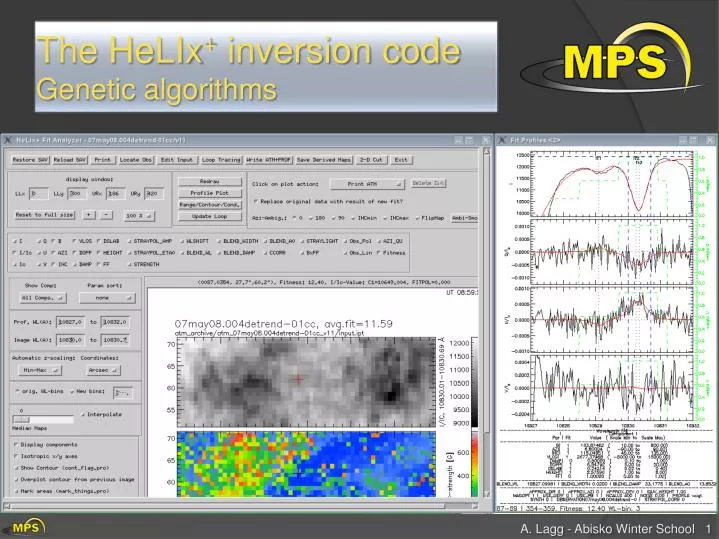
The HeLIx + inversion code Genetic algorithms. Inversion of the RTE. Once solution of RTE is known: comparison between Stokes spectra of synthetic and observed spectrum trial-and-error changes of the initial parameters of the atmosphere („human inversions“)

E N D
Inversion of the RTE Once solution of RTE is known: comparison between Stokes spectra of synthetic and observed spectrum trial-and-error changes of the initial parameters of the atmosphere(„human inversions“) until observed and synthetic (fitted) profile matches Inversions:Nothing else but an optimization of the trial-and-error part Problem:Inversions always find a solution within the given model atmosphere. Solution is seldomly unique (might even be completely wrong). Goal of this lecture:Principles of genetic algorithmsLearn the usage of the HeLIx+ inversion code, develop a feeling on the reliability of inversion results.
The merit function The quality of the model atmosphere must be evaluated Stokes profiles represent discrete sampled functions widely used: chisqr definition • weight(also WL-dep) • sum over WL-pixels • sum over Stokes • number of free parameters • RTE gives the Stokes spectrum Issyn • The unknowns of the system are the (height dependent) model parameters:
HeLIx+ overview of features • includes Zeeman, Paschen-Back, Hanle effect (He 10830) • atomic polarization for He 10830 (He D3) • magneto-optical effects • fitting / removing telluric lines • fitting unknown parameters of spectral lines • various methods for continuum correction / fitting • convolution with instrument filter profiles • user-defined weighting scheme • direct read access to SOT/SP, VTT-TIP2, SST-CRISP, ... • flexible atomic data configuration • extensive IDL based display routines • MPI support (to invert maps) Download from http://www.mps.mpg.de/homes/laggGBSO download-section helixuse invert and IR$soft
steepest gradient Pikaia The inversion technique: reliability Two minimizations implemented: Levenberg-Marquardt: requires good initial guess PIKAIA (genetic algorithm, Charbonneau 1995): no initial guess needed planned: DIRECT algorithm (good compromise between global min and speed)
Initial guess problem Having a good initial guess for the iteration process improves both the speed and the convergence of the inversion.
Initial guess optimizations Weak field initialization Auer77 initialization • Other methods: • Artificial Neural Networks (ANN) • MDI / magnetograph formulae • use a minimization technique which does not rely on initial guess values
Genetic algorithms Genetic algorithms (GA’s) are a technique to solve problems which need optimization GA’s are a subclass of Evolutionary Computing GA’s are based on Darwin’s theory of evolution History of GA’s: Evolutionary computing evolved in the 1960’s. GA’s were created by John Holland in the mid-70’s. P. Spijker, TU Eindhoven
Advantages / drawbacks No derivatives of the goodness of fit function with respect to model parameters need be computed; it matters little whether the relationship between the model and its parameters is linear or nonlinear. Nothing in the procedure outlined above depends critically on using a least-squares statistical estimator; any other robust estimator can be substituted, with little or no changes to the overall procedure. In most real applications, the model will need to be evaluated (i.e., given a parameter set, compute a synthetic dataset and its associated goodness of fit) a great many times; if this evaluation is computationally expensive, the forward modeling approach can become impractical.
Evolution in biology Each cell of a living thing contains chromosomes - strings of DNA Each chromosome contains a set of genes - blocks of DNA Each gene determines some aspect of the organism (like eye colour) A collection of genes is sometimes called a genotype A collection of aspects (like eye colour) is sometimes called a phenotype Reproduction involves recombination of genes from parents and then small amounts of mutation (errors) in copying The fitness of an organism is how much it can reproduce before it dies Evolution based on “survival of the fittest”
Biological reproducion During reproduction “errors” occur Due to these “errors” genetic variation exists Most important “errors” are: Recombination (cross-over) Mutation
Natural selection The origin of species: “Preservation of favourable variations and rejection of unfavourable variations.” There are more individuals born than can survive, so there is a continuous struggle for life. Individuals with an advantage have a greater chance for survive: survival of the fittest. Important aspects in natural selection are: adaptation to the environment isolation of populations in different groups which cannot mutually mate If small changes in the genotypes of individuals are expressed easily, especially in small populations, we speak of genetic drift “success in life”: mathematically expressed as fitness
How to apply to RTE? GA’s often encode solutions as fixed length “bitstrings” (e.g. 101110, 111111, 000101) Each bit represents some aspect of the proposed solution to the problem For GA’s to work, we need to be able to “test” any string and get a “score” indicating how “good” that solution is definition of “fitness function” required: convenient to use chisqr merit functionGA’s improve the fitness – maximization technique David Hales (www.davidhales.com)
Road 0 500 1000 Solution1 = 300 Solution2 = 900 Example – Drilling for oil Imagine you had to drill for oil somewhere along a single 1km desert road Problem: choose the best place on the road that produces the most oil per day We could represent each solution as a position on the road Say, a whole number between [0..1000] David Hales (www.davidhales.com)
Encoding problem The set of all possible solutions [0..1000] is called the search space or state space In this case it’s just one number but it could be many numbers or symbols Often GA’s code numbers in binary producing a bitstring representing a solution In our example we choose 10 bits which is enough to represent 0..1000 In GA’s these encoded strings are sometimes called “genotypes” or “chromosomes” and the individual bits are sometimes called “genes”
Fitness of oil function Solution1 = 300 (0100101100) Solution2 = 900 (1110000100) Road 0 1000 O I L 30 5 Location
Search space Oil example: search space is one dimensional (and stupid: how to define a fitness function?). RTE: encoding several values into the chromosome many dimensions can be searched Search space an be visualised as a surface or fitness landscape in which fitness dictates height (fitness / chisqrhypersurface) Each possible genotype is a point in the space A GA tries to move the points to better places (higher fitness) in the space
Search space Obviously, the nature of the search space dictates how a GA will perform A completely random space would be bad for a GA Also GA’s can, in practice, get stuck in local maxima if search spaces contain lots of these Generally, spaces in which small improvements get closer to the global optimum are good
The algorithm Generate a set of random solutions Repeat Test each solution in the set (rank them) Remove some bad solutions from set Duplicate some good solutions make small changes to some of them Until best solution is good enough How to duplicate good solutions?
Adding Sex Two high scoring “parent” bit strings (chromosomes) are selected and with some probability (crossover rate) combined Producing two new offsprings(bit strings) Each offspring may then be changed randomly (mutation) Selecting parents: many schemes possible, example:Roulette Wheel Add up the fitness's of all chromosomes Generate a random number R in that range Select the first chromosome in the population that - when all previous fitness’s are added - gives you at least the value R sex result of sex parents are seldom happy with the result
Roulette Wheel Selection 1 2 3 4 5 6 7 8 1 2 3 1 3 5 1 2 0 18 Rnd[0..18] = 7 Chromosome4 Parent1 Rnd[0..18] = 12 Chromosome6 Parent2 Higher chance of picking a fit chromosome!
Crossover - Recombination 1011011111 1010000000 Parent1 Offspring1 1010000000 1001011111 Offspring2 Parent2 Crossover single point - random With some high probability (crossover rate) apply crossover to the parents. (typical values are 0.8 to 0.95)
Mutation mutate 1011001111 1011011111 Offspring1 Offspring1 1000000000 1010000000 Offspring2 Offspring2 Original offspring Mutated offspring With some small probability (the mutation rate) flip each bit in the offspring (typical values between 0.1 and 0.001)
Improved algorithm Generate a population of random chromosomes Repeat (each generation) Calculate fitness of each chromosome Repeat Use roulette selection to select pairs of parents Generate offspring with crossover and mutation Until a new population has been produced Until best solution is good enough
Many Variants of GA Different kinds of selection (not roulette):Tournament, Elitism, etc. Different recombination:one-point crossover, multi-point crossover, 3 way crossover etc. Different kinds of encoding other than bitstringInteger values, Ordered set of symbols Different kinds of mutationvariable mutation rate Different reduction planscontrols how newly bred offsprings are inserted into the population PIKAIA (Charbonneau, 1995)
List ofME Codes (incomplete) HeLIx+A. Lagg, most flexible code (multi-comp, multi line), He 10830 Hanle slab model implemented. Genetic algorithm Pikaia. Fully parallel. VFISVJ.M.Borrero, for SDO HMI. Fastest ME code available. F90, fully parallel. Levenberg-Marquardt with some optimizations. MERLINWritten by Jose Garcia at HAO in C, C++ and some other routines in Fortran. (Lites et al. 2007 in Il Nouvo Cimento) MELANIEHector Socas at HAO. In F90, not parallel. Numerical derivatives. HAZELArtoro Lopez Ariste et al. (2008). Optimized for He 10830, He D3, Hanle-slab model. MILOSOrozco Suarez et al. (2007), IDL, some papers published with it
Installation & Usage of HeLIX+ Follow instructions on user‘s manual: • Basic usage: • 1-component model, create & invert synthetic spectrum • discuss problems: • parameter crosstalk • uniqueness of solution • stability & reliability • influence of noise Download from http://www.mps.mpg.de/homes/laggGBSO download-section helixuse invert and IR$soft
Exercise II:HeLIx+ installation and basic usage • install and run IDL interface of HeLIx+ • the first input file: synthesis of Fe I 6302.5 • change atmospheric parameters (B, INC, …) • change line parameters (quantum numbers, geff) • display Zeeman pattern • add noise • 1st inversion • play with noise level / initial values / parameter range • weighting scheme • Synthesis • add complexity to atmospheric model (stray-light, multi-component) • add 2nd spectral line (Fe 6301.5) • blind tests: • take synthetic profile from someone else and invert it • Which parameters are robust? • How can robustness be improved? Download first input file: abisko_1c.ipt http://www.mps.mpg.de/homes/lagg/