Download
1 / 23
240 likes | 363 Views
SRNWP-NT mini workshop in Toulouse 12-13 December 2002. A cell-integrated semi-Lagrangian dynamical scheme based on a step-function representation. Eigil Kaas, Bennert Machenhauer and Peter Hjort Lauritzen Danish Meteorological Institute Lyngbyvej 100, DK-2100 Copenhagen, Denmark.

E N D
SRNWP-NT mini workshop in Toulouse 12-13 December 2002 A cell-integrated semi-Lagrangian dynamical scheme based on a step-function representation Eigil Kaas, Bennert Machenhauer and Peter Hjort Lauritzen Danish Meteorological Institute Lyngbyvej 100, DK-2100 Copenhagen, Denmark
The goals • To construct a dynamical scheme for atmospheric dynamics and tracer transport with all the following properties: • Indefinite order of accuracy for advection by a flow that is constant in time an space (except for initial truncation). • Full local mass conservation. • Positive definite. • Monotonic. • Numerically effective. • Our solution: SF-CISL • Step-Function Cell Integrated Semi-Lagragian scheme combined with a semi-implicit scheme for inertia-gravity wave terms.
OUTLINE • The basic idea behind step function advection. • The basic idea behind CISL. • 2-D passive test simulations. • A new semi-implicit formulation of CISL for the shallow water equations. • Tests simulations. • Discussion: efficiency, generalisation to 3-D and to spherical geometry …
What is CISL ? Integrate the continuity equation over a time dependent Lagrangian volume: Nair and Machenhauer (2002)
What is CISL ? Nair and Machenhauer (2002)
The basic idea behind step-function advection i-1 i i+1 x-direction Time
3. Calculate the ‘s and define the re-mappings. 6. Calculate for each ”north-south” intersect Order of calculations 1. Calculate dxi,j and dyi,j for each Eulerian grid cell. 2. Calculate the departure grid cell corner points. 4. Perform the cell integration (result = ) 5. Calculate for each departure grid cell point corner point 7. Calculate for each departure cell (=(result of 4.)/) 8. Do the ”horizontal diffusion” (i.e. modify if needed)
11. Use this information to calculate the final value of 12. Calculate the final values of and from the values of dxi,j , dyi,j and . Order of calculations (cont.) 9. Calculate new values of dxi,j and dyi,j based on upstream values of , and . 10. Calculate the relative areal change for each step function
2-D passive test simulations Solid body rotation, 6 rotations, 96 time steps per rotation 100 x 100 grid points/cells
A new semi-implicit formulation of CISL for the shallow water equations. depth of fluid height of topography velocity components
A new semi-implicit 2-D CISL formulation (1) The traditional two-time level SL-scheme: ~ indicates time extrapolation from n and n-1 CISL explicit forecast: Ideal semi-implicit CISL forecast: Elliptic equation too complicated !
A new semi-implicit 2-D CISL formulation (2) The basic explicit forecast Inconsistent implicit correction term Correction of the inconsistency in the previous time step
Tests of the semi-implicit SF-CISL in a shallow water channel model 20000 km 20000 km
Four different model formulatoins • Eulerian grid-point model: • 3 time level centered difference scheme • Semi-implicit formulation (Coriolis explicit) • Reasonable explicit horizontal diffusion • Spectral Eulerian model: • 3 time level spectral transform scheme (double Fourier series) • Semi-implicit formulation (Coriolis explicit) • Reasonable implicit horizontal diffusion • Interpolating semi-Lagrangian (IPSL) model: • 2 time level scheme based on bi-cubic interpolation • Semi-implicit formulation (Coriolis implicit) • No additional horizontal diffusion • SF-CISL model: • 2 time level scheme based on step-function representation • Semi-implicit formulation (Coriolis implicit) • No additional horizontal diffusion
48 hour ”forecasts” at low resolution. Parameter: height field Spectral Eulerian model Eulerian grid-point model Interpol. semi Lagrangian model SF-CISL model
48 hour ”forecasts” at high resolution. Parameter: height field Spectral Eulerian model Eulerian grid-point model Interpol. semi Lagrangian model SF-CISL model
48 hour ”forecasts” at low resolution. Parameter: passive tracer Spectral Eulerian model Eulerian grid-point model SF-CISL model Interpol. semi Lagrangian model
48 hour ”forecasts” at high resolution. Parameter: passive tracer Spectral Eulerian model Eulerian grid-point model SF-CISL model Interpol. semi Lagrangian model
10 day ”forecasts” at high resolution. Parameter: passive tracer Interpol. semi Lagrangian model SF-CISL model
Discussion and conclusion • Cost • Passive advection 1.7 times IPSL. • Truncation/horizontal diffusion • This is a critical point • Memory consumption • When step function geometries are defined from the total mass field they could in principle be used for all prognostic variables (i.e. only one prognostic variable per tracer variable) ”Bad” • The passive advection tests in realistic flow demonstrate the monotonicity, mass conservation and positive definiteness • The shallow-model works with the new scheme ! • No noise due to step functions ”Good”
Discussion and conclusion • Other possible formulations • “horizontal diffusion/truncation” • Choice of step-functions. • Generalisation to 3-D • Cascade interpolation (Nair et al. 1999) for the vertical problem. • Prognostic variables: 3-D cell averages, horizontal averages at model levels, vertical averages at grid points, grid point values. • Spherical geometry • No real problem (reduced lat-lon (or Gaussian) grid).