Download
1 / 52
530 likes | 981 Views
Structural Health Monitoring. Sukun Kim, David Culler James Demmel, Gregory Fenves, S teve G laser Thomas Oberheim, Shamim Pakzad UC Berkeley. NEST Retreat – Jun 4, 2004. Structure Monitoring. Data Acquisition. Data Collection. Processing & Feedback. Overview.

E N D
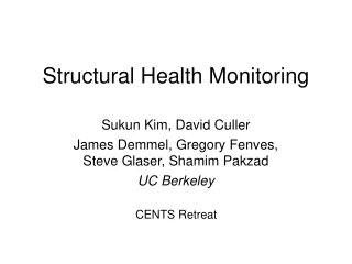
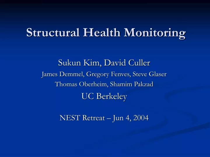
Structural Health Monitoring Sukun Kim, David Culler James Demmel, Gregory Fenves, Steve Glaser Thomas Oberheim, Shamim Pakzad UC Berkeley NEST Retreat – Jun 4, 2004
Structure Monitoring Data Acquisition Data Collection Processing & Feedback
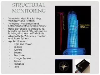
Overview • Low cost structure monitoring - Monitor structure, and analyze the health of structure based on sensed data at low cost • For Golden Gate Bridge, monitor vibration of bridge, and detect unusual behavior by wind, earthquake, or local damage • Extend reach of Wireless Sensor Network in a different direction – high fidelity sampling • High accuracy, high frequency with low jitter, large amount of data
Challenges • Data Acquisition • Accelerometer Board • High Frequency Sampling & Jitter • Data Collection • Large-scale Reliable Data Transfer • Signal processing & System Identification
Accelerometer Board • Both accelerometers for two axis • Thermometer • 16bit ADC
Sampling Other job Non-preemptible portion (atomic section) Preemptible task portion 0μs 10μs Jitter Histogram HighFrequencySampling
Receiver Sender Open Ack for Open Data Block 1 Data Block 2 Data Block 3 Data Block 4 Ack for Data DONE DONE Large-scale Reliable Transfer • Explicit open handshake - Data description and size of cluster is sent as a transfer request • Data transfer is composed of multiple rounds. In each round, sender sends packets missing in the previous round • Tear-down is implicit
Throttle for data packet is fixed at 10 pkt/s • Optimal case: window size is infinite • For the case with window size 16, throughput is 88% of optimal case. • Considering loss rate of 3%, actual relative throughput is 91%, which is higher than 85% of channel utilization ratio. This is because control packets do not follow 10 packets/s.
Status • Measure acceleration from multiple boards synchronously • Sather tower • PowerBar building • Data is available on the web
Signal Processing and System Identification • Signal Processing • Analog low-pass filter with threshold frequency 25Hz is used • Averaging is used. If noise follows Gaussian distribution, by averaging N numbers, noise decreases by a factor of sqrt(N) • System Identification • Identifying model of target system • By matching input to system and output from system, construct a mathematical system model (Box-Jenkins multi-input multi-output model)
Large Scale Earthquake G G Accelerometer variation Acoustic Noise mG mG Traffic Identification Local Damage Detection Temperature μG μG Nuclear Test Detection Gravity Variation nG nG Challenges versus Accuracy Possible Applications versus Accuracy Conclusion • New challenges are analyzed which are brought by structure monitoring to wireless sensor network • High accuracy accelerometer, high frequency sampling with low jitter, low-pass filter, averaging, large-scale reliable data collection
Table of Contents • Overview • Data Acquisition • Accelerometer Board • High Frequency Sampling & Jitter • Data Collection • Large-scale Reliable Data Transfer • Signal processing & System Identification • Conclusion • Challenges & Future Work
HighFrequencySampling • Made by David Gay • Up to 6.67KHz with 4 bytes sample • MicroTimer – Supports one timer, micro second level granularity • BufferLog – Has two buffers. One is filled up by upper layer application while the other buffer is written to flash memory as a background task
Jitter Test (1KHz, 5KHz, 6.67KHz) • Peak to Peak is time to fill up buffer • Spiky portion is time to write buffer to flash • Can sample as long as the former is larger than the latter
Jitter Test Histogram(1KHz, 5KHz, 6.67KHz) • Jitter is within 10µs • Peak at 625ns – Wakeup time from sleep mode
Sampling Sample Other job Non-preemptible portion (atomic section) Preemptible task portion F(k2) F(k3) . . . C C+T(k1) C+T(k2) Jitter Jitter Analysis
Table of Contents • Overview • Data Acquisition • Accelerometer Board • High Frequency Sampling & Jitter • Data Collection • Large-scale Reliable Data Transfer • Signal processing & System Identification • Conclusion • Challenges & Future Work
Large-scale Reliable Data Transfer • 4Byte of data and 4Byte of time stamp at 100Hz in 100 nodes, transfer 40pkt/s – Sample data for 5 minutes, and collect data for more than 5 hours!!! • Efficient and reliable data transfer is crucial • RAM to RAM one-hop transfer is implemented as a building block - LRX
Receiver Sender Open Ack for Open Data Block 1 Data Block 2 Data Block 3 Data Block 4 Ack for Data DONE DONE LRX component (continued) • Explicit open handshake - Data description and size of cluster is sent as a transfer request • Data transfer is composed of multiple rounds. In each round, sender sends packets missing in the previous round • Tear-down is implicit
Throttle for data packet is fixed at 10 pkt/s • Optimal case: window size is infinite • For the case with window size 16, throughput is 88% of optimal case. • Considering loss rate of 3%, actual relative throughput is 91%, which is higher than 85% of channel utilization ratio. This is because control packets do not follow 10 packets/s.
As loss rate increases, retransmission increases, and throughput decreases
Channel Utilization • LRX (data only) is the theoretical limit of LRX (when window size is infinite) • Usage LRX lowers channel utilization by 15%
Table of Contents • Overview • Data Acquisition • Accelerometer Board • High Frequency Sampling & Jitter • Data Collection • Large-scale Reliable Data Transfer • Signal processing & System Identification • Conclusion • Challenges & Future Work
Signal Processing • As an analog signal processing low-pass filter is used, which filters high frequency noise • For accelerometer board, low-pass filter with threshold frequency 25Hz is used. Then ADC should sample at frequency much higher than 50Hz by Nyquist theorem, and imperfect low-pass filter • As a digital signal processing, averaging is used. If noise follows Gaussian distribution, by averaging N numbers, noise decreases by a factor of sqrt(N)
System Identification • Identifying model of target system • By matching input to system and output from system, we can construct a mathematical system model. • Usual process is (1) fitting a general Box-Jenkins multi-input multi-output model to sampled data. (2) And natural frequencies, damping ratios and mode shape are then estimated using the estimated Box-Jenkins model. • Most part of system identification is under development on civil engineering side.
Table of Contents • Overview • Data Acquisition • Accelerometer Board • High Frequency Sampling & Jitter • Data Collection • Large-scale Reliable Data Transfer • Signal processing & System Identification • Conclusion • Challenges & Future Work
Large Scale Earthquake G G Accelerometer variation Acoustic Noise mG mG Traffic Identification Local Damage Detection Temperature μG μG Nuclear Test Detection Gravity Variation nG nG Challenges versus Accuracy Possible Applications versus Accuracy Conclusion • New challenges are analyzed which are brought by structure monitoring to wireless sensor network • High accuracy accelerometer, high frequency sampling with low jitter, low-pass filter, averaging, large-scale reliable data collection
Table of Contents • Overview • Data Acquisition • Accelerometer Board • High Frequency Sampling & Jitter • Data Collection • Large-scale Reliable Data Transfer • Signal processing & System Identification • Conclusion • Challenges & Future Work
Challenges & Future Work • Calibrating acceleration value to temperature • Time synchronization – RBS, TPSN • To maximize utility of channel, we need to monitor channel quality (loss rate), and throttle packet injection rate accordingly • Using LRX as a building block, multi-hop data collection need be implemented • TASK
Cost Comparison • Conventional piezoelectric accelerometer with PC system costs $40,000 • Budget for structure monitoring budget is $1,000,000 level • Wireless sensor network with MEM accelerometer costs $500 • Cheaper by a factor of 100
Shaking Table Test • Silicon Design 1221L is more quite, but less sensitive to dynamic movement
Noise Floor Test • Blue – Seismic Vault • Red – McCone Hall
Sample F(k2) F(k3) . . . C C+T(k1) C+T(k2) Jitter Jitter Analysis (continued) • T(i): execution time of atomic section i • X(i): a random variable uniformly distributed in [0, T(i)] • C: context switch time • F(i): frequency of occurrence of atomic section i • Assume that the probability of timer event occurring at any point in atomic section i is same, then jitter will follow C+X(i). • Since jitter distribution of every atomic section begins from C, the frequency is highest near C and decreases as moving farther. And frequency drop at C+T(i) by F(i), since atomic section i will not have any distribution beyond C+T(i). • Actually there is a peak at C, because when program is in preemptible section, it will immediately service timer event after context switch time C.
Calculation of Transfer Timer • Let us assume each node store 4Byte of data and 4Byte of time stamp at 100Hz. And assume there are 100 nodes, radio throughput is 1.2KB/s, and data is collected to one base station. If acceleration data worthy 5 minutes is collected, each node will transfer 240,000Bytes. 100 nodes will transfer 24,000,000Bytes. Since the end link to base station is a bottleneck, it will take more than 5 hours. We can see bandwidth is narrow compared to aggressive data sampling. Even if we alleviate this problem using multi-channel or multi-tier network, still we will be in short of bandwidth.
LRX component • Transfers one data cluster, which is composed of several blocks. • One block fits into one packet, so the number of blocks is equal to window size. • Each data cluster has a data description. After looking at data description, receiver may deny data (receiver already has that data, or that data is not useful anymore).
Receiver Sender Open Ack for Open Data Block 1 Data Block 2 Data Block 3 Data Block 4 Ack for Data DONE DONE
Receiver Sender Open Open Ack for Open Data Block 1 Data Block 2
Receiver Sender Open Ack for Open Open Ack for Open Data Block 1 Data Block 2
Receiver Sender Data Block 1 Data Block 2 Data Block 3 Data Block 4 Ack for Data Data Block 2 Ack for Data DONE DONE
Receiver Sender Data Block 1 Data Block 2 Data Block 3 Data Block 4 Ack for Data DONE Data Block 4 Ack for Data DONE
Receiver Sender Data Block 1 Data Block 2 Data Block 3 Data Block 4 Data Block 4 Ack for Data DONE DONE
Receiver Sender Data Block 1 Data Block 2 Data Block 3 Data Block 4 Ack for Data Data Block 2 Ack for Data Data Block 3
Why Sender times out • There are two reasons why only sender times out and stimulate receiver for Ack. The first reason is shown in Figure 16. If sender doesn’t time out, for a receiver to make sure Ack is delivered to sender, receiver should get acknowledgement from sender for Ack itself. This is not good. So it is clear that sender should timeout. Given that sender times out, timeout of receiver makes no difference except that channel is wasted by unnecessary Ack from receiver. So timeout in only sender side is desirable. As a second reason, if receiver times out, in case like Figure 18 (if first Data after Ack is lost), second Data always collide with resent Ack of receiver. This is not a good phenomenon. Therefore, after sending last packet in each round, if acknowledgement does not come, sender sends the last packet in that round again to stimulate acknowledgement. However, this does not mean receiver has no timeout. Receiver waits sufficient amount of time, and if nothing happens, it regards the situation as a failure.
Amplitude Frequency Filtering threshold Imperfect Low-pass Filter
Time Synchronization • Temporal jitter is handled by high frequency sampling component. Spatial jitter should be solved by time synchronization. ITP [8] is a time synchronization protocol widely used in Internet. In wireless sensor network, there were several studies. In RBS [9], synchronization is done among receivers, eliminating sender’s jitter in media access. TPSN [10] put time stamp after obtaining channel. This gives even better synchronization accuracy than RBS (10μs compared to 20μs). Still there is a source of jitter at receiver side. As we saw in jitter for sampling, handling interrupt by radio can be delayed by atomic section of other activity. As suggested in [10], putting time stamp at MAC layer in receiver side will eliminate this jitter.


![Global Trend & Forecast Structural Health Monitoring [2020]](https://cdn4.slideserve.com/7242416/slide1-dt.jpg)