Download
1 / 77
790 likes | 1.03k Views
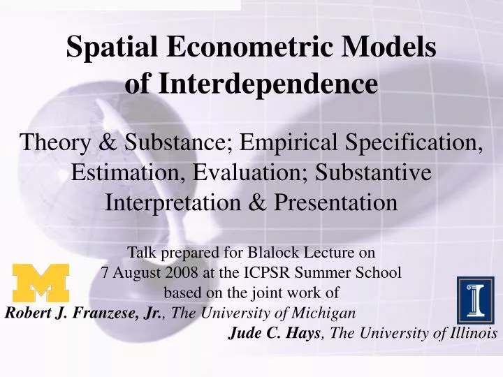
Spatial Econometric Models of Interdependence Theory & Substance; Empirical Specification, Estimation, Evaluation; Substantive Interpretation & Presentation. Talk prepared for Blalock Lecture on 7 August 2008 at the ICPSR Summer School based on the joint work of

E N D
Spatial Econometric Modelsof InterdependenceTheory & Substance; Empirical Specification, Estimation, Evaluation; Substantive Interpretation & Presentation Talk prepared for Blalock Lecture on 7 August 2008 at the ICPSR Summer School based on the joint work of Robert J. Franzese, Jr., The University of Michigan Jude C. Hays, The University of Illinois
Overview • Motivation: Integration & Domestic Policy-Autonomy • Does economic integration constrain govts from redistributing income, risk, & opportunity through tax & spending policies? • In answering this & related questions, scholars have overlooked spatial interdependence of domestic policies as important evidence. • Economic integration generates externalities across political jurisdictions, which implies strategic policy interdependence, so policy of one govt will be influenced by policies of its neighbors. • Interdependence Substance, Theory, & Empirics: Use contexts econ integration (& related) to explore & explain: • Substance:i’s actions depend on j’s. Examples. • Theory: • General: externalitiesstrategic policy complements/substitutesrace-to-bottom/top/elseearly/late-mover advantagesstrategic delay/rush-for-1st • Specific: a model of inter-jurisdictional tax-competition (P&T ch. 12) • Empirics: “Galton’s Problem”; Estimation, Inference, Interpretation, & Presentation
A Motivating Context:Globalization & Domestic-Policy Autonomy • Standard Argument: • ↑ capital mobility & trade integration sharpen capital’s threat vs. domestic govts to flee excessive/inefficient tax & public policy; forces welfare-state retrench & tax shift from more-mob. cap. (esp. finance) to less-mob. lab. (esp. skilled-man.) • Recent counter-arguments & findings: • Some empirical Q whether constrained or ° constraint from trade/capital integ. • Counter-arguments (e.g.): • Rodrik (Cameron): Demand (contra supply) SocPol may ↑ w/ integ indeterminate • Garrett ’98/Boix ’98: Left/active govt more/as efficient capital not flee • Hall-Soskice ‘01/Franzese-Mosher ’02: comparative institutional advantage trade-integ foster divergence; (liquid) cap-integ may foster race to bottom (not nec’ly) zero • Swank ’02 (& many others): political & economic barriers &/or advantages considerable maneuvering room • Standard & all counter arguments spatial interdependence b/c whatever pressures may arise from globalization depend on what neighbors, competitors, partners, substitutes, & complements do • Accordingly, appropriate model places others’ policies on right-hand side • Basinger-Hallerberg ’04 maybe 1st in C&IPE to notice & incorporate explicitly • Interdependence (def):yi=f(yj≠i); note: not merely that yi & yj≠i corr
The Broad Range of Spatial Interdependence • (Simmons et al.’s 06) Mechanisms: • Competition • Coercion • Learning • Emulation • [Migration/Contagion (F&H Add)] • Theoretical Contexts (ubiquitous): • ANY Strategic Decision-making: sisj • Externalities & Spillovers • Learning/Emulation, Demonstration • Networks/Epistemic Communities • Literal Diffusion, Contagion, Migration • Substantive Contexts (ubiquitous): • Security Policy (e.g., alliances, wars) • Environmental (e.g., air-pollution reg) • Regulatory (e.g., telecomm stds) • Legis reps’ votes depend on others’ • Elects., cand. qualities or strategies • p(∙)&outs coups (Li&Thompson 75), riots (Govea&West 81), revolts (Brinks&Copp 06) • Contextual effects in micro-behavior: • Braybeck&Huckfeldt 02ab, Cho 03, Huckfeldt et al. 05, Cho&Gimpel 07, Cho&Rudolph 07, Lin et al 06 • Policy, instit’s, regimes diffusion: • Policy: Schneider&Ingram‘88, Rose ‘93, Meseguer ‘04,‘05, Gilardi ‘05 • Institutional or regime: Implicit/Informal: Dahl’s Polyarchy, Starr’s Democratic Dominoes, Huntington’s 3rd Wave. Explicit/Formal: O’Loughlin et al. ‘98, Brinks & Coppedge ‘06, Gleditsch & Ward ‘06, ’07 • Int’l diffusion of liberalization: • Simmons&Elkins 04, 06a, 06b, Eising 02, Brune et al. 04, Brooks 05… • Globalization & interdependence: • Genschel 02, Basinger&Hallerberg 04, Knill 05, Jahn 06, Swank 06, F&H 06,07, Kayser 07 • Tobler’s Law: ‘‘I invoke the first law of geography: everything is related to everything else, but near things are more related than distant things’’ (1970). • Plus: “Space More Than Geography” (Beck, Gleditsch, & Beardsley 2006)
Substantive & Theoretical Ubiquity & Centrality (1) • US State Policy-innovation diffusion: deep roots & much contemporary interest, & sustained attention between: • Crain 1966; Walker 1969, 1973; Gray 1973; Knoke 1982; Caldiera 1985; Lutz 1987; Berry & Berry 1990; Case et al. 1993; Berry 1994; Rogers 1995; Mintrom 1997ab; Brueckner 1998; Mintrom & Vergari 1998; Mossberger 1999; Berry & Berry 1999; Godwin & Schroedel 2000; Balla 2001; Mooney 2001; Wejnert 2002; Coughlin et al. 2003; Bailey & Rom 2004; Boehmke & Witmer 2004; Daley & Garand 2004; Grossback et al. 2004; Mencken 2004; Berry & Baybeck 2005; Garrett et al. 2005; Costa-Font & Ons-Novell 2006; Karch 2006; Rincke 2006; Shipan & Volden 2006; Volden 2006; Werck et al. 2006; Woods 2006; Volden et al. 2007. • Similar policy-learning mechanisms underlie some comparative studies of policy diffusion: • Schneider & Ingram 1988; Rose 1993; Bennett 1997; Dolowitz & Marsh 2000; True & Mintrom 2001; Tews et al. 2003; Jensen 2004; Meseguer 2004, 2005; Brooks 2005, 2007; Gilardi 2005; Gilardi et al. 2005; Murillo & Schrank 2005; Weyland 2005; Braun & Gilardi 2006; Linos 2006; Parys 2006; Ermini & Santolini 2007; Moscone et al. 2007. • Institutional or regime diffusion likewise long-standing & recently much reinvigorated: • Dahl’s 1971 Polyarchy (1 of 8 causes dem listed); center-stage Starr’s 1991 “Democratic Dominoes”; Huntington’s 1991 Third Wave; Beissinger 2007; Bunce & Wolchik 2006, 2007; et al. in E. Eur. Transitions; Hagopian & Mainwaring 2005 et al. in LA; O’Loughlin et al. 1998, Brinks & Coppedge 2006, Gleditsch & Ward 2006, 2007 estimated empirically extent, paths, &/or patterns dem diffuse. Kelejian et al. 2007 give institutional diffusion general theoretical & empirical treatment. • C&IPE, e.g. globalization≈interdependence: • Diffusion of “Liberalization” & Related: Simmons & Elkins 2004, Simmons et al. 2006, Eising 2002; Brune et al. 2004; Brooks 2005, 2007; Jordana & Levi-Faur 2005; Way 2005; Lazer 2006; Prakash & Potoski 2006; Brune & Guisinger 2007; and many others. • Glob/Interdep/TaxComp & Dom Policy Auton: Genschel 2002; Guler et al. 2002; Franzese & Hays 2003, 2004b, 2005a, 2007abc, 2008c; Badinger et al. 2004; Basinger & Hallerberg 2004; Heichel et al. 2005; Henisz et al. 2005; Holzinger & Knill 2005; Knill 2005; Polillo & Guillén 2005; Elkins et al. 2006; Jahn 2006; Lee & Strang 2006; Manger 2006; Swank 2006; Baturo & Grey 2007; Cao 2007; Cao et al. 2007; Coughlin et al. 2007; Garretsen & Peeters 2007; Mosley & Uno 2007; Mukherjee & Singer 2007.
Substantive & Theoretical Ubiquity & Centrality (2) • Representatives’ votes (Lacombe & Shaughnessy 2005), citizens’ votes (Huckfeldt & Sprague 1991; O’Laughlin et al. 1994; Pattie & Johnston 2000; Beck et al. 2003; Calvo & Escolar 2003; Kim et al. 2003; Schofield et al. 2003; Lacombe & Shaughnessy 2007), election outcomes (Shin & Agnew 2002, 2007; Hiskey & Canache 2005; Wing & Walker 2006; Kayser 2007), candidate qualities, contributions, or strategies (Goldenberg et al. 1986; Mizruchi 1989; Krasno et al. 1994; Cho 2003; Gimpel et al. 2006) • Probabilities & outcomes of coups (Li & Thompson 1975), riots (Govea & West 1981), civil wars (Murdoch & Sandler 2004, Buhaug & Rød 2006) &/or revolutions (Brinks & Coppedge 2006) • IR: interdep≈definition of subject: • States’ entry into wars, alliances, treaties (Murdoch et al. 2003), or organizations. • Empirical attention to inherent spat-dep IR greatest in: Shin & Ward 1999; Gleditsch & Ward 2000; Gleditsch 2002; Ward & Gleditsch 2002; Hoff & Ward 2004; Gartzke & Gleditsch 2006; Salehyan & Gleditsch 2006; Gleditsch 2007, and, in different way, Signorino 1999, 2002, 2003; Signorino & Yilmaz 2003; Signorino & Tarar 2006 • In micro-behavioral work, too, long-standing & surging interest “contextual” or “neighborhood” effects: • Huckfeldt & Sprague 1993 review, some of which stress interdep: Straits 1990; O’Loughlin et al. 1994; Knack & Kropf 1998; Liu et al. 1998; Braybeck & Huckfeldt 2002ab; Beck et al. 2002; McClurg 2003; Huckfeldt et al. 2005; Cho & Gimpel 2007; Cho & Rudolph 2007. Sampson et al. 2002 and Dietz 2002 review the parallel large literature on neighborhood effects in sociology • At & beyond other disciplinary borders, subjects include: • Social-movements: McAdam & Rucht 1993; Conell & Cohn 1995; Giugni 1998; Strang & Soule 1998; Biggs 2003; Browning et al. 2004; Andrews & Biggs 2006; Holmes 2006; Swaroop & Morenoff 2006. • Microeconomic preferences: Akerloff 1997; Postlewaite 1998; Glaeser & Scheinkman 2000; Manski 2000; Brock & Durlauf 2001; Durlauf 2001; Glaeser et al. 2003; Yang & Allenby 2003; Sobel 2005; Ioannides 2006; Soetevent 2006 • Macroeconomic performance: Fingleton 2003; Novo 2003; Kosfeld & Lauridsen 2004; Maza & Villaverde 2004; Kelejian et al. 2006; Mencken et al. 2006 • Technology, marketing, and other firm strategies: Abramson & Rosenkopf 1993; Geroski 2000; Strang & Macy 2001; Holloway 2002; Bradlow 2005; Autant-Berard 2006; Mizruchi et al. 2006 • Violence and crime: Grattet et al. 1998; Myers 2000; Baller et al. 2001; Morenoff et al. 2001; Villareal 2002; Baker & Faulkner 2003; Oberwittler 2004; Bhati 2005; Mears & Bhati 2006; Brathwaite & Li 2008 • Fertility, birthweight, child development, & child poverty: Tolnay 1995 and Montgomery & Casterline 1996; Morenoff 2003; Sampson et al. 1999; Voss et al. 2006 • Not to mention public health and epidemiology (contagion!). • More exotic topics: ordainment of women (Chaves 1996), right-wing extremism (Rydgren 2005), marriage (Yabiku 2006), national identity (Lin et al. 2006), & faculty (Weinstein 2007).
Policy Interdependence:A General Theoretical Model (Brueckner ‘03) • i’s utility depends pi & pj b/c interdep (& vv): • Accordingly, i’s optimal policy, pi*, depends j’s action, pj: • So slope best-response function depends on effect of pj on marginal utility of pi: • Therefore: Diminishing returns and… • …negative externalities =>strategic complements: • Positive slope: positive feedback/same-signed reactions • …positive externalities => strategic substitutes: • Negative slope: neg. feedback/opposite-signed reactions
Policy Interdependence:General Theory & Substantive Implications • Dimin returns & neg externalities Strategic Complements • Race-to-Bottom (RTB) (or -Top). Examples: • Tax Competition • Labor Regulation • Trade Barriers (politically) • Early-mover advantage “race to go first” • E.g.: Exch.Deprec., tech.stds. (& other focal pts. in coord. or battle sexes) • Dimin returns & pos externalities Strategic Substitutes • Free-Riding Incentives • E.g., Alliance Security: • E.g., ALMP: • Late-mover advantage strategic delay & Wars of Attrition • DimRet & both +&– externs: • Environmental Reg’s (& CHIPs?):
Figure 2. Best Response Functions: Strategic Substitutes p2 p1
An International Tax-Competition Model as a Specific Substantive Example of Interdependence • Stylized Theoretical Model Cap-Tax Comp. (P&T ‘00, ch.12) • 2 jurisdicts, dom & for cap-tax, τk & τk* to fund fixed spend. For-invest mobility costs, M. • Inds’ lab-cap endow, ei, & choose lab-leisure, l & x, & save-invest, s=k+f to max ω=U(c1)+c2+V(x), over l, c1, & c2, s.t. time-c., 1+ei=l+x, & b.c.’s, 1–ei=c1+k+f+≡c1+s & c2=(1–τk)k+(1–τk*)f–M(f)+(1–τl)l. • equilibrium economic choices of citizens: • indirect utility, W, defined over policy variables, τl, τk, & τk*: • Besley-Coate (‘97) citizen-candidate(s) face(s) electorate w/ these prefs. • Stages: 1) elects, 2) cit-cand winners set taxes, 3) all private econ decisions made. • Ebm win cand has endow eP such that desires implement this Modified Ramsey Rule: • Best-Response Functions: τk=T(eP,τk*) & τk*=T*(eP*,τk) for dom & for pm. • Slopes: ∂T/∂τk* & ∂T*/∂τk, pos or neg b/c ↑τk* cap-inflow; can use ↑tax-base to ↓τk or to ↑τk (seizing upon ↓elasticity base). • Background of this slide plots case both positively sloped; illustrated comparative static is of leftward shift of domestic government.
Empirical Models of Interdependence:Galton’s Problem in C&IPE • Interdependence yi=f(yj) • Generic (linear) dynamic spatial-lag model of C&IPE: • Galton’s Problem: Extremely difficult disting why C(yi,yj) b/c... • 1. Correlated domestic/unit-level conditions, d (CPE) • 2. Common/corr’d exposure exog-external shocks/conditions, s (open-CPE) • 3. Responses to these 2 may be context-conditional, sd (CC-CPE) • 40. Correlated stochastic component (Beck-Katz), nuisance C&IPE • 4. Interdependence/diffusion/contagion: yi=f(yj,CC-CPE), substance C&IPE • Upshot Empirically (Franzese & Hays ‘03,‘04,‘06ab,‘07abcd,‘08ab): • ° omit or mis-specify CPE, tend over-estimate IPE (interdependence) & v.v. • yiyj => textbook endogeneity/simultaneity problem w/ spatial lag; analogous: • ° fail redress endog sufficiently mis-est (usu. over-est.) ρ (under)mis-est. β • Most Important Conclusion:Model It!TM Insofar as omit or rel’ly mis-spec spatial interdep, tend over-est impact domestic & exog-ext factors & v.v. most crucial, regardless of CPE/IPE emphasis: well-spec model & measure both. • S-OLS may suffice. OVB >> simultaneity bias in any of practical examples we’ve considered, & S-OLS did OK our MCs provided interdep remained modest (|ρ|<.3±).
The Terms of Galton’s Problem:Omitted-Variable vs. Simultaneity Biases inSpatial- and Spatio-Temporal-Lag Models • OVB (rel. mis-spec.) v. simultaneity: • OVB (OLS): • SimB (S-OLS): • In S-T, little more complicated, but: With all positive S-T dep, ρ space-dep over-est’d & time-dep & β under-est’d
Estimating Spatial/Spatio-Temporal-Lag Models • Inconsistent Estimators: • Omit spatial-dep (e.g., OLS): bad idea if ρ non-negligible • Ignore simultaneity (e.g., S-OLS): could be OK (in MSE) if ρ not too large & sample-dims benevolent • Simplest Option, if Available: • Time-Lagged Spatial-Lag OLS easy & unbiased iff… • No contemporaneous (i.e., w/in obs period) interdependence. • Model of temporal dynamics sufficiently accurate (see Achen) • 1st obs pre-determined; if not, spatial-Hurwicz bias (order 1/T) • Consistent Estimators • S-IV/2SLS/GMM: Use WX to instrument Wy, etc. • S-ML: Specify system for Max-Likelihood estimation
Estimating Spatial- & Spatio-Temporal-Dynamic Models by S-ML • S-ML for Spatial-Lag Model: • Std, but ε → y by |A| not 1 computational issues, plus • Conditional S-ML S-T (ie., given 1stobs, Nx1 form); (unconditional is messy but exists; won’t show): • Stationarity (if row-stdzd, & ρ,>0): ρ+<1 • Spatial Probit: complicated but doable (show if time) • m-STAR & Est’d W; endog W: doable (show if…)
APPLICATIONS • Globalization, Tax Competition, & Domestic Policy • Replicates: Swank&Steinmo 02, Hays 03, Basinger&Hallerberg 04 • ALMP: Active-Labor-Market Policy in EU (F&H ‘06) • DepVar: LMT spend per unemployed worker • Hypoth: Positive spillovers (@ borders) effective member-state ALMP free-riding & underinvest. Appreciable? • IndVars: rGDPpc, UE, UDen, Deindustrialization (Iversen-Soskice), Trade, FDI, Pop65, LCab, CDemCab, LLibVote, GCons • MIDs & Trade: Beck, Gleditsch, & Beardsley ’06 • DepVar: Directed trade data; • Hypoth: MIDs affect trade in & beyond dyad • IndVars: GDPab, POPab, Distance, tau-b, MutualDem, MID, Bi/MultiPoleSys • AFDC & CHIPs in U.S. States (Volden ’06) • AFDC: Hypoth—“states as laboratories”≈diffusion by learning • DepVar: max monthly AFDC benefit • Ind Vars: state’s poverty rate, avg monthly wage in retail, govt ideology (0-100, R-L), º interparty competition (.5-1.0, comp-non), tax effort (rev as % tax capacity), & % AFDC bens paid by fed govt. • CHIPs: Hypoth—“states as laboratories”≈diffusion by learning • DepVar: 1 if state’s CHIP includes monthly premium; IndVars same.
Practical Model Specification & Estimation • Most convenient to work in (Nx1) vector form: • WN=an NxN of (time-invariant) spatial wts, wij, & WNIT gives W. • E.g., 15x15 binary-contiguity from ALM paper: • N.b., row-stdz typ., convenient, but not nec’ly subst’ly neutral • Ideally, substance, which not nec’ly geography, in W. • Beware of extant software: critical bug in LeSage’s MatLab code; likelihood in some third-party Stata SAR code seems flat wrong.
Interpreting Spatial/Spatio-Temporal Effects • The Model: • Model may look linear, but is not; as in all beyond purely linear-additive, coefficients & effects very different things! • Convenient, for interpretation, to write model this way too: • Coefficients, βx are just pre-spatial, pre-temporal—and wholly unobservable!—impulse from some x to y. • Spatio-Temporal Effects: • Post-spatial, pre-temporal “instantaneous effect” of x: • Spatio-Temporal Response Paths: • LR Multiplier/LR-SS:
Presenting Spatial/Spatio-Temporal Effects • Standard Errors (Confidence Intervals & Hypothesis Tests) of Effects: • Delta Method: • …or Simulate! • Upshot: Cannot see substance clearly from only the estimated coefficients & their standard errors • Effective Presentational Options: • SR/LR-Response Grids • Spatio-Temporal Response-Paths • Maps
Conclusion • Spatial & Spatio-Temporal Interdependence • Important & Appreciable Substance (e.g., globalization & int’l cap-tax compete seems quite real & does constrain), not Nuisance. • Therefore: Model them. Interpret them. • How specify & estimate models? • If space-lag is time-lagged, not problem; but if thry & substance says immediate (w/in an observational period), can handle that too: • S-OLS not a bad strategy even then, if ρ not too big & smpl-dims right; S-ML, & in some regards IV-based strategies, seem effective • Spatio-Temporal Effects not directly read from coefficients: use graphs & maps & grids • Information-demands of Galton’s Problem severe • Standard errors of effects tend big. Suspect delta-method lin-approx. maybe part problem; plan explore performance bootstrap. • Max effort & care theory, measure, specification, to both C&IPE
Spatial QualDep: The Econometric Problem (1) • Spatial Qualitative/Categorical/Lmtd-Dep-Var Models in the Lit: • Spatial probit: McMillen 1992,1995; Bolduc et. al. 1997; Pinkse & Slade 1998; LeSage 1999, 2000; Beron et al. 2003; Beron & Vijverberg 2004 • Spatial logit: Dubin 1997; Lin 2003; Autant-Bernard 2006 • Spatial sample-selection (i.e., s-Tobit/Heckit): McMillen 1995, Smith & LeSage 2004, Flores-Lagunes & Schnier 2006 • Spatial multinomial-probit: McMillen 1995, Bolduc et al. 1997 • Spatial discrete-duration: Phaneuf & Palmquist 2003 • Survival w/ spatial frailty: Banerjee et al. 2004, Darmofal 2007 • Spatial count: Bhati 2005, including ZIP: Rathbun & Fei 2006 • The Challenge: • Not n indep., unidimensional CDF std normals, so (log-)likelihood=product (sum) thereof, but 1 n-dimensional CDF of non-std (heterosked.) normals • Spatial Latent-Variable Models: Estimation Strategies • McMillen 1992: EM algorithm, rendered spatial probit estimable, but no std-errs & arb. parameterization of induced heteroscedasticity. • McMillen 1995, Bolduc et. al. 1997: simulated-likelihood strategies to estimate spatial-MNP • Beron et al. ‘03, Beron & Vijverberg ‘04: recursive-importance-sampling (RIS) estimator • LeSage 1999, 2000: Bayesian strategy of Markov-Chain-Monte-Carlo (MCMC) by Metropolis-Hastings-within-Gibbs sampling. • Fleming 2004: simpler, if approximate, strategies allowing interdep. in (non)linear probability models, estimable by NLS, GLM, or GLMM • Pinkse & Slade’s 1998: two-step GMM estimator (for spatial-error probit).
The Econometric Problem (2) • Structural Model: • Reduced Form: • Measurement Equation: • Probability: • Or: • For Spatial-Error-Probit:
The Econometric Problem (3) • Comments: • Notice that, when we come to interpret & , we face the same MVN integration • We haven’t seen such substantive interpretation yet attempted fully in the literature, but we suggest an easier way to do it. • If can order dependence pattern & ensure only antecedent y* appear on RHS, then std probit ML w/ a spatial-lag works • We think usu. indefensible subst’ly/thry’ly, but cf. Swank on capital-tax competition, e.g., where argues US exclusively leads & omits US. • Having y, not y*, on RHS may seem subst’ly or thry’ly desirable in some cases, but gen’ly not logically possible: • Problem would be that outcome, yi, would indirectly (via spatial feedback) determine yi*, but then yi* would directly determine yi. The stochastic difference b/w them will thus a logical inconsistency. • Notice similar MVN issue w/ time lags; suggests similar strategies (but simpler b/c ordered) may allow model temp dynamics directly rather than nuisance (e.g., BKT splines)
The Estimators: Bayesian Gibbs-MH Sampler (1) • Basic Idea (See Gill’s intro Bayesian textbook, e.g.): • Monte Carlo (MC): Given likelihood/posterior, can sample to estimate any quantity of interest, including density, e.g. • Markov Chain (MC)MC: • Each draw depends on previous, so need only conditional like./post. • Some theorems indicate, under fairly gen’l conditions, distribution parameter draws converges to distribution under true like./post. • Gibbs Sampler: simplest of MCMC family: • Express each parameter like./post. conditional on others. • Cycle to draw each conditional on others’ starts or previous draw • After some sufficient “burn-in”, all subsequent param-vector draws follow true multivariate likelihood/posterior. • Metropolis-Hastings: useful when cond’l param-dist non-std • Draws from a seed or jump distribution are accepted or rejected as the next sampled parameters, depending on how they compare to a suitably transformed expression of the target distribution