Download

1 / 35
360 likes | 524 Views
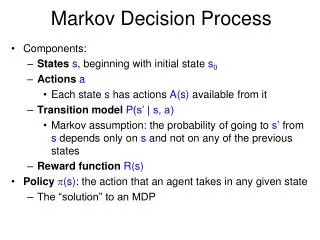
Markov Decision Process (MDP). Ruti Glick Bar-Ilan university. Policy. Policy is similar to plan generated ahead of time Unlike traditional plans, it is not a sequence of actions that an agent must execute If there are failures in execution, agent can continue to execute a policy

E N D
Markov Decision Process(MDP) Ruti Glick Bar-Ilan university
Policy • Policy is similar to plan • generated ahead of time • Unlike traditional plans, it is not a sequence of actions that an agent must execute • If there are failures in execution, agent can continue to execute a policy • Prescribes an action for all the states • Maximizes expected reward, rather than just reaching a goal state
Utility and Policy • utility • Compute for every state • “What is the usage (utility) of this state for the overall task?” • Policy • Complete mapping from states to actions • “In which state should I perform which action?” • policy: state action
The optimal Policy π*(s) = argmaxa∑s’T(s, a, s’)U(s’) T(s, a, s’) = Probability of reaching state s from state s U(s’) = Utility of state j. • If we know the utility we can easily compute the optimal policy. • The problem is to compute the correct utilities for all states.
Finding π* • Value iteration • Policy iteration
Value iteration • Process: • Calculate the utility of each state • Use the values to select an optimal action
+1 -1 START Bellman Equation • Bellman Equation: • U(s) = R(s) + γmaxa ∑ (T(s, a, s’) U(s’)) • For example:U(1,1) = -0.04+γmax{ 0.8U(1,2)+0.1U(2,1)+0.1U(1,1), 0.9U(1,1)+0.1U(1,2), 0.9U(1,1)+0.1U(2,1), 0.8U(2,1)+0.1U(1,2)+0.1U(1,1,) } Up Left Down Right
Bellman Equation • properties • U(s) = R(s) + γ maxa ∑ (T(s, a, s’) U(s’)) • n equations. One for each step • n vaiables • Problem • Operator max is not a linear operator • Non-linear equations. • Solution • Iterative approach
Value iteration algorithm • Initial arbitrary values for utilities • Update utility of each state from it’s neighbors • Ui+1(s) R(s) + γmaxa ∑ (T(s, a, s’) Ui(s’)) • Iteration step called Bellman update • Repeat till converges
Value Iteration properties • This equilibrium is a unique solution! • Can prove that the value iteration process converges • Don’t need exact values
convergence • Value iteration is contraction • Function of one argument • When applied on to inputs produces value that are “closer together • Have only one fixed point • When applied the value must be closer to fixed point • We’ll not going to prove last point • converge to correct value
Value Iteration Algorithm function VALUE_ITERATION (mdp) returns a utility function input:mdp, MDP with states S, transition model T, reward function R, discount γ local variables:U, U’ vectors of utilities for states in S, initially identical to R repeat U U’ for each state s in S do U’[s] R[s] + γmaxa s’ T(s, a, s’)U[s’] untilclose-enough(U,U’) return U
Example • Small version of our main example • 2x2 world • The agent is placed in (1,1) • States (2,1), (2,2) are goal states • If blocked by the wall – stay in place • The reward are written in the board
Example (cont.) • First iteration • U(1,1) = R(1,1) + γ max { 0.8U(1,2) + 0.1U(1,1) + 0.1U(2,1), 0.9U(1,1) + 0.1U(1,2), 0.9U(1,1) + 0.1U(2,1), 0.8U(2,1) + 0.1U(1,1) + 0.1U(1,2)} = -0.04 + 1 x max { 0.8x(-0.04) + 0.1x(-0.04) + 0.1x(-1), 0.9x(-0.04) + 0.1x(-0.04), 0.9x(-0.04) + 0.1x(-1), 0.8x(-1) + 0.1x(-0.04) + 0.1x(-0.04)} =-0.04 + max{ -0.136, -0.04, -0.136, -0.808} =-0.08 • U(1,2) = R(1,2) + γ max {0.9U(1,2) + 0.1U(2,2), 0.9U(1,2) + 0.1U(1,1), 0.8U(1,1) + 0.1U(2,2) + 0.1U(1,2), 0.8U(2,2) + 0.1U(1,2) + 0.1U(1,1)}= -0.04 + 1 x max {0.9x(-0.04)+ 0.1x1, 0.9x(-0.04) + 0.1x(-0.04), 0.8x(-0.04) + 0.1x1 + 0.1x(-0.04), 0.8x1 + 0.1x(-0.04) + 0.1x(-0.04)} =-0.04 + max{ 0.064, -0.04, 0.064, 0.792} =0.752 • Goal states remain the same
Example (cont.) • Second iteration • U(1,1) = R(1,1) + γ max { 0.8U(1,2) + 0.1U(1,1) + 0.1U(2,1), 0.9U(1,1) + 0.1U(1,2), 0.9U(1,1) + 0.1U(2,1), 0.8U(2,1) + 0.1U(1,1) + 0.1U(1,2)} = -0.04 + 1 x max { 0.8x(0.752) + 0.1x(-0.08) + 0.1x(-1), 0.9x(-0.08) + 0.1x(0.752), 0.9x(-0.08) + 0.1x(-1), 0.8x(-1) + 0.1x(-0.08) + 0.1x(0.752)} =-0.04 + max{ 0.4936, 0.0032, -0.172, -0.3728} =0.4536 • U(1,2) = R(1,2) + γ max {0.9U(1,2) + 0.1U(2,2), 0.9U(1,2) + 0.1U(1,1), 0.8U(1,1) + 0.1U(2,2) + 0.1U(1,2), 0.8U(2,2) + 0.1U(1,2) + 0.1U(1,1)}= -0.04 + 1 x max {0.9x(0.752)+ 0.1x1, 0.9x(0.752) + 0.1x(-0.08), 0.8x(-0.08) + 0.1x1 + 0.1x(0.752), 0.8x1 + 0.1x(0.752) + 0.1x(-0.08)} =-0.04 + max{ 0.7768, 0.6688, 0.1112, 0.8672} = 0.8272
Example (cont.) • Third iteration • U(1,1) = R(1,1) + γ max { 0.8U(1,2) + 0.1U(1,1) + 0.1U(2,1), 0.9U(1,1) + 0.1U(1,2), 0.9U(1,1) + 0.1U(2,1), 0.8U(2,1) + 0.1U(1,1) + 0.1U(1,2)} = -0.04 + 1 x max { 0.8x(0.8272) + 0.1x(0.4536) + 0.1x(-1), 0.9x(0.4536) + 0.1x(0.8272), 0.9x(0.4536) + 0.1x(-1), 0.8x(-1) + 0.1x(0.4536) + 0.1x(0.8272)} =-0.04 + max{ 0.6071, 0.491, 0.3082, -0.6719} =0.5676 • U(1,2) = R(1,2) + γ max {0.9U(1,2) + 0.1U(2,2), 0.9U(1,2) + 0.1U(1,1), 0.8U(1,1) + 0.1U(2,2) + 0.1U(1,2), 0.8U(2,2) + 0.1U(1,2) + 0.1U(1,1)}= -0.04 + 1 x max {0.9x(0.8272)+ 0.1x1, 0.9x(0.8272) + 0.1x(0.4536), 0.8x(0.4536) + 0.1x1 + 0.1x(0.8272), 0.8x1 + 0.1x(0.8272) + 0.1x(0.4536)} =-0.04 + max{ 0.8444, 0.7898, 0.5456, 0.9281} = 0.8881
Example (cont.) • Continue to next iteration… • Finish if “close enough” • Here last change was 0.114 – close enough
“close enough” • We will not go down deeply to this issue! • Different possibilities to detect convergence: • RMS error –root mean square error of the utility value compare to the correct values demand of RMS(U, U’) < ε when: ε – maximum error allowed in utility of any state in an iteration
“close enough” (cont.) • Policy Loss :difference between the expected utility using the policy to the expected utility obtain by the optimal policy || Ui+1– Ui || < ε (1-γ) / γ When: ||U|| = maxa |U(s)| ε – maximum error allowed in utility of any state in an iteration γ – the discount factor
Finding the policy • True utilities have founded • New search for the optimal policy: For each s in S doπ[s] argmaxa ∑s’ T(s, a, s’)U(s’) Return π
Example (cont.) • Find the optimal police • Π(1,1) = argmaxa { 0.8U(1,2) + 0.1U(1,1) + 0.1U(2,1), //Up 0.9U(1,1) + 0.1U(1,2), //Left 0.9U(1,1) + 0.1U(2,1), //Down 0.8U(2,1) + 0.1U(1,1) + 0.1U(1,2)} //Right = argmaxa { 0.8x(0.8881) + 0.1x(0.5676) + 0.1x(-1), 0.9x(0.5676) + 0.1x(0.8881), 0.9x(0.5676) + 0.1x(-1), 0.8x(-1) + 0.1x(0.5676) + 0.1x(0.8881)} = argmaxa { 0.6672, 0.5996, 0.4108, -0.6512} = Up • Π(1,2) = argmaxa { 0.9U(1,2) + 0.1U(2,2), //Up 0.9U(1,2) + 0.1U(1,1), //Left 0.8U(1,1) + 0.1U(2,2) + 0.1U(1,2), //Down 0.8U(2,2) + 0.1U(1,2) + 0.1U(1,1)} //Right = argmaxa { 0.9x(0.8881)+ 0.1x1, 0.9x(0.8881) + 0.1x(0.5676), 0.8x(0.5676) + 0.1x1 + 0.1x(0.8881), 0.8x1 + 0.1x(0.8881) + 0.1x(0.5676)} = argmaxa {0.8993, 0.8561, 0.6429, 0.9456} = Right
0.812 0.868 0.912 +1 +1 +1 +1 0.762 0.660 -1 -1 -1 -1 0.705 0.655 0.611 0.388 Summery – value iteration 1. The given environment 2. Calculate utilities 4. Execute actions 3. Extract optimal policy
Example - convergence Error allowed
Policy iteration • picking a policy, then calculating the utility of each state given that policy (value iteration step) • Update the policy at each state using the utilities of the successor states • Repeat until the policy stabilize
Policy iteration • For each state in each step • Policy evaluation • Given policy πi. • Calculate the utility Ui of each state if π were to be execute • Policy improvement • Calculate new policy πi+1 • Based on πi • π i+1[s] argmaxa ∑s’ T(s, a, s’)U(s’)
Policy iteration Algorithm function POLICY_ITERATION (mdp) returns a policy input:mdp, an MDP with states S, transition model T local variables:U, U’ vectors of utilities for states in S, initially identical to R π, a policy, vector indexed by states, initially random repeat U Policy-Evaluation(π,U,mdp) unchanged? true for each state s in Sdo if maxa s’T(s, a, s’) U[s’] > s’T(s, π[s], s’) U[s’] then π[s] argmaxa s’T(s, a, s’) U[j] unchanged? false end until unchanged? returnπ
Example • Back to our last example… • 2x2 world • The agent is placed in (1,1) • States (2,1), (2,2) are goal states • If blocked by the wall – stay in place • The reward are written in the board • Initial policy: Up (for every step)
Example (cont.) • First iteration – policy evaluation • U(1,1) = R(1,1) + γ x (0.8U(1,2) + 0.1U(1,1) + 0.1U(2,1)) U(1,2) = R(1,2) + γ x (0.9U(1,2) + 0.1U(2,2)) U(2,1) = R(2,1) U(2,2) = R(2,2) • U(1,1) = -0.04 + 0.8U(1,2) + 0.1U(1,1) + 0.1U(2,1) U(1,2) = -0.04 + 0.9U(1,2) + 0.1U(2,2) U(2,1) = -1 U(2,2) = 1 • 0.04 = -0.9U(1,1) + 0.8U(1,2) + 0.1U(2,1) + 0U(2,2)0.04 = 0U(1,1) – 0.1U(1,2) + 0U(2,1) + 0.1U(2,2)-1 = 0U(1,1) + 0U(1,2) - 1U(2,1) + 0U(2,2) 1 = 0U(1,1) + 0U(1,2) - 0U(2,1) + 1U(2,2) • U(1,1) = 0.3778 U(1,2) = 0.6 U(2,1) = -1 U(2,2) = 1 Policy Π(1,1) = Up Π(1,2) = Up
Example (cont.) Policy Π(1,1) = Up Π(1,2) = Up • First iteration – policy improvement • Π(1,1) = argmaxa { 0.8U(1,2) + 0.1U(1,1) + 0.1U(2,1), //Up 0.9U(1,1) + 0.1U(1,2), //Left 0.9U(1,1) + 0.1U(2,1), //Down 0.8U(2,1) + 0.1U(1,1) + 0.1U(1,2)} //Right = argmaxa { 0.8x(0.6) + 0.1x(0.3778) + 0.1x(-1), 0.9x(0.3778) + 0.1x(0.6), 0.9x(0.3778) + 0.1x(-1), 0.8x(-1) + 0.1x(0.3778) + 0.1x(0.6)} = argmaxa { 0.4178, 0.4, 0.24, -0.7022} = Up don’t have to update • Π(1,2) = argmaxa { 0.9U(1,2) + 0.1U(2,2), //Up 0.9U(1,2) + 0.1U(1,1), //Left 0.8U(1,1) + 0.1U(2,2) + 0.1U(1,2), //Down 0.8U(2,2) + 0.1U(1,2) + 0.1U(1,1)} //Right= argmaxa { 0.9x(0.6)+ 0.1x1, 0.9x(0.6) + 0.1x(0.3778), 0.8x(0.3778) + 0.1x1 + 0.1x(0.6), 0.8x1 + 0.1x(0.6) + 0.1x(0.3778)} = argmaxa { 0.64, 0.5778, 0.4622, 0.8978} = Right update
Example (cont.) • Second iteration – policy evaluation • U(1,1) = R(1,1) + γ x (0.8U(1,2) + 0.1U(1,1) + 0.1U(2,1)) U(1,2) = R(1,2) + γ x (0.1U(1,2) + 0.8U(2,2) + 0.1U(1,1)) U(2,1) = R(2,1) U(2,2) = R(2,2) • U(1,1) = -0.04 + 0.8U(1,2) + 0.1U(1,1) + 0.1U(2,1) U(1,2) = -0.04 + 0.1U(1,2) + 0.8U(2,2) + 0.1U(1,1) U(2,1) = -1 U(2,2) = 1 • 0.04 = -0.9U(1,1) + 0.8U(1,2) + 0.1U(2,1) + 0U(2,2)0.04 = 0.1U(1,1) – 0.9U(1,2) + 0U(2,1) + 0.8U(2,2)-1 = 0U(1,1) + 0U(1,2) - 1U(2,1) + 0U(2,2) 1 = 0U(1,1) + 0U(1,2) - 0U(2,1) + 1U(2,2) • U(1,1) = 0.5413 U(1,2) = 0.7843 U(2,1) = -1 U(2,2) = 1 Policy Π(1,1) = Up Π(1,2) = Right
Example (cont.) • Second iteration – policy improvement • Π(1,1) = argmaxa { 0.8U(1,2) + 0.1U(1,1) + 0.1U(2,1), //Up 0.9U(1,1) + 0.1U(1,2), //Left 0.9U(1,1) + 0.1U(2,1), //Down 0.8U(2,1) + 0.1U(1,1) + 0.1U(1,2)} //Right = argmaxa { 0.8x(0.7843) + 0.1x(0.5413) + 0.1x(-1), 0.9x(0.5413) + 0.1x(0.7843), 0.9x(0.5413) + 0.1x(-1), 0.8x(-1) + 0.1x(0.5413) + 0.1x(0.7843)} = argmaxa { 0.5816, 0.5656, 0.3871, -0.6674} = Up don’t have to update • Π(1,2) = argmaxa { 0.9U(1,2) + 0.1U(2,2), //Up 0.9U(1,2) + 0.1U(1,1), //Left 0.8U(1,1) + 0.1U(2,2) + 0.1U(1,2), //Down 0.8U(2,2) + 0.1U(1,2) + 0.1U(1,1)} //Right= argmaxa { 0.9x(0.7843)+ 0.1x1, 0.9x(0.7843) + 0.1x(0.5413), 0.8x(0.5413) + 0.1x1 + 0.1x(0.7843), 0.8x1 + 0.1x(0.7843) + 0.1x(0.5413)} = argmaxa {0.8059, 0.76, 0.6115, 0.9326} = Right don’t have to update Policy Π(1,1) = Up Π(1,2) = Right
Example (cont.) • No change in the policy has found finish • The optimal policy:π(1,1) = Upπ(1,2) = Right • Policy iteration must terminate since policy’s number is finite
Simplify Policy iteration • Can focus of subset of state • Find utility by simplified value iteration:Ui+1(s) = R(s) + γ∑s’ (T(s, π(s), s’) Ui(s’)) OR • Policy Improvement • Guaranteed to converge under certain conditions on initial polity and utility values
Policy Iteration properties • Linear equation – easy to solve • Fast convergence in practice • Proved to be optimal
Value vs. Policy Iteration • Which to use: • Policy iteration in more expensive per iteration • In practice, Policy iteration require fewer iterations