Download
1 / 56
560 likes | 756 Views
9 . Atmospheric neutrinos and Neutrino oscillations (Cap. 11-12 book). Corso “ Astrofisica delle particelle ” Prof. Maurizio Spurio Università di Bologna a.a . 2014/15. Outlook. Some history Neutrino Oscillations How do we search for neutrino oscillations Atmospheric neutrinos

E N D
9.Atmospheric neutrinos and Neutrino oscillations(Cap. 11-12 book) Corso “Astrofisica delle particelle” Prof. Maurizio Spurio Università di Bologna a.a. 2014/15
Outlook • Some history • Neutrino Oscillations • How do we search for neutrino oscillations • Atmospheric neutrinos • 10 years of Super-Kamiokande • Upgoing muons and MACRO • Interpretation in terms on neutrino oscillations • Appendix: The Cherenkov light
Once upon a time… • At the beginning of the ’80s, some theories (GUT) predicted the proton decay with measurable livetime • The proton was thought to decay in (for instance) pe+p0ne • Detector size: 103 m3, and mass 1kt (=1031 p) • The main background for the detection of proton decay were atmospheric neutrinos interacting inside the experiment • Water CerenkovExperiments (IMB, Kamiokande) • Trackingcalorimeters (NUSEX, Frejus, KGF) • Result: NO p decay ! But some anomalies on the neutrino measurement! gg Neutrino Interaction e Proton decay
Neutrino Oscillations • Idea of neutrinos being massive was first suggested by B. Pontecorvo • Prediction came from proposal of neutrino oscillations Neutrinos are created or annihilated as W.I. eigenstates |ne , |nm , |nt=Weak Interactions (WI) eigenstats |n1 , |n2 , |n3=Mass (Hamiltonian)eigenstats • Neutrinos propagate as a superposition of mass eigenstates
Weak eigenstates(e, , )are expressedas a combinations of the mass eigenstates(1, 2,3). • These propagate with different frequencies due to their different masses, and different phases develop with distance travelled. Let us assume two neutrino flavors only. • The time propagation: |n(t)= (|n1 , |n2 ) (eq.1) M = (2x2 matrix) (eq.2)
Time propagation eq.1 becames, using eq.2) (eq.4) (eq.5) whose solution is : with During propagation, the phase difference is: (eq.6)
Time evolution of the “physical” neutrino states: • Let us assume two neutrino flavors only (i.e. the electon and the muon neutrinos). • They are linear superposition of the n1,n2 eigenstaten: |ne=cosq|n1+ sinq|n2 |nm=-sinq|n1+ cosq|n2 q = mixing angle (eq.3) • Using eq. 5 in eq. 3, we get: (eq.7)
At t=0, eq. 7 becomes: (eq.8) • By inversion of eq. 8: (eq.9) • For the experimental point of view (accelerators, reactors), a pure muon (or electron) state a t=0 can be prepared. For a purenmbeam, eq. 9: (eq.10)
The time evolution of thenmstate of eq. 8: (eq.11) By definition, the probability that the state at a given time is anmis: (eq. 12) • Using eq. 11, the probability: (eq. 13) i.e. using trigonometry rules: (eq. 14)
Finally, using eq.5: (eq. 15) With the following substitutions in eq.15: - the neutrino path length L=ct (in Km) - the mass difference Dm2 = m22 – m12 (in eV2) - the neutrino Energy En (in GeV) (eq. 16) To see “oscillations” pattern:
..with atmospheric neutrinos • Dm2, sin22Q from Nature; • En= experimental parameter (energy distribution of neutrino giving a particular configuration of events) • L = experimental parameter (neutrino path length from production to interaction)
The recipes for the evaluation of the atmospheric neutrino flux- \
i) The primary spectrum E < 1015 eV Galactic 5. 1019 < E< 3. 1020 eV E-3 spectrum 1015 < E< 1018 eV galactic ? GZK cut E 5. 1019 eV Extra-Galactic? Unexpected?
ii)- CR-air cross section It needs a model of nucleus-nucleus interactions Average number of charged hadrons produced in pp (andpp) collisions versus center of mass energy pp Cross section versus center of mass energy.
iii) Model of the atmosphere • ATMOSPHERIC NEUTRINO PRODUCTION: • high precision 3D calculations, • refined geomagnetic cut-off treatment (also geomagnetic field in atmosphere) • elevation models of the Earth • different atmospheric profiles • geometry of detector effects
Output: the neutrino (ne,nm) flux Seeforinstance the FLUKA MC: http://www.mi.infn.it/~battist/neutrino.html
n Through goingm n m m n iv) The Detector response Partially Contained Stoppingm Fully Contained m n Energy spectrum of n for each event category Energy spectrum (from Monte Carlo) of atmospheric neutrinos seen with different event topologies (SuperKamiokande) up-stop m up-thru m
Rough estimate: how many ‘Contained events’ in 1 kton detector 1. Flux: Fn ~ 1 cm-2 s-1 2. Cross section (@ 1GeV): sn~0.5 10-38 cm2 3. Targets M= 6 1032 (nucleons/kton) 4. Time t= 3.1 107 s/y nm ne Nint = Fn(cm-2 s-1) x sn(cm2)x M (nuc/kton) x t (s/y) ~ ~ 100 interactions/ (kton y)
15 years of Super-Kamiokande 1996.4 Start data taking 1998 Evidence of atmospheric n oscillation (SK) SK-I 1999.6 K2K started 2001 Evidence of solar n oscillation (SNO+SK) 2001.7 data taking was stopped for detector upgrade 2001.11 Accident partial reconstruction 2002.10 data taking was resumed SK-II 2005 Confirm n oscillation by accelerator n (K2K) 2005.10 data taking stopped for full reconstruction SK-III 2006.7 data taking was resumed 2009 data taking SK-IV
Measurement of contained events and SuperKamiokande (Japan) • 1000 m Deep Underground • 50.000 ton of Ultra-Pure Water • 11000 +2000 PMTs • Working since 1996
Cherenkov Radiation • As a charged particle travels, it disrupts the local electromagnetic field (EM) in a medium. • Electrons in the atoms of the medium will be displaced and polarized by the passing EM field of a charged particle. • Photons are emitted as an insulator's electrons restore themselves to equilibrium after the disruption has passed. • In a conductor, the EM disruption can be restored without emitting a photon. • In normal circumstances, these photons destructively interfere with each other and no radiation is detected. • However, when the disruption travels faster than light is propagating through the medium, the photons constructively interfere and intensify the observed Cerenkov radiation.
b>1/n b<1/n Effetto Cerenkov Per unatrattazioneclassicadell’effetto Cerenkov: Jackson : Classical Electrodynamics, cap 13 e par. 13.4 e 13.5 La radiazione Cerenkov e’ emessa ogniqualvolta una particella carica attraversa un mezzo (dielettrico) con velocita’bc=v>c/n, dove v e’ la velocita’ della particella e n l’indice di rifrazione del mezzo. Intuitivamente: la particella incidente polarizza il dielettrico gli atomi diventano dei dipoli. Se b>1/n momento di dipolo elettrico emissione di radiazione.
L’ angolo di emissione qcpuo’ essere interpretato qualitativamente come un’onda d’urto come succede per una barca od un aereo supersonico. Esiste una velocità di soglia bs = 1/n qc ~ 0 Esiste un angolo massimo qmax=arcos(1/n) La cos(q) =1/bn e’ valida solo per un radiatore infinito, e’ comunque una buona approssimazione ogniqualvolta il radiatore e’ lungo L>>lessendo l la lunghezza d’onda della luce emessa
Numero di fotoniemessi per unitàdi percorso e intervallodi lunghezzad’onda. Osserviamochedecresce al crescere della l Il numero di fotoniemessi per unita’ di percorso non dipendedallafrequenza
L’ energiapersa per radiazione Cerenkov cresce con b. Comunqueanche con b 1 e’ molto piccola. Molto piu’ piccola di quellapersa per eccitazione/ionizzazione (Bethe Block), al massimo 1% .
Esisteunasoglia per emissione di luce Cerenkov • La luce e’ emessa ad un angoloparticolare Facile utilizzarel’effetto Cerenkov per identificare le particelle. Con 1) possosfruttare la soglia Cerenkov a soglia. Con 2) misurarel’angolo DISC, RICH etc. La luceemessa e rivelabile e’ poca. Consideriamo un radiatorespesso 1 cm un angoloqc = 30oed un DE = 1 eVedunaparticella di carica 1. Considerandoinoltrechel’efficienzaquantica di un fotomoltiplicatore e’ ~20% Npe=18 fluttuazionialla Poisson
Cherenkov Radiation One of the 13000 PMTs of SK
Contained event in SuperKamiokande Fully Contained (FC) Partially Contained (PC) m e or m Reduction No hit in Outer Detector One cluster in Outer Detector Automatic ring fitter Particle ID Energy reconstruction Fiducial volume (>2m from wall, 22 ktons) Evis > 30 MeV (FC), > 3000 p.e. (~350 MeV) (PC) Fully Contained 8.2 events/day Evis<1.33 GeV : Sub-GeV Evis>1.33 GeV : Multi-GeV Partially Contained 0.58 events/day
Contained events. The up/down symmetry in SK andnm/neratio. Up/Down asymmetry interpreted as neutrino oscillations En=0.5GeV En=3 GeV En=20 GeV Expectations: events inside the detector. For En> a few GeV, Upward / downward = 1
DATA m / e Data = 0.638 0.017 0.050 m / e M C Zenith angle distribution SK:1289 days (79.3 kty) • Electron neutrinos = DATA and MC (almost) OK! • Muon neutrinos = Large deficit of DATA w.r.t. MC ! Zenith angle distributions for e-like and µ-like contained atmospheric neutrino events in SK. The lines show the best fits with (red) and without (blue) oscillations; the best-fit is Dm2= 2.0 × 10⁻³ eV2 and sin2 2θ = 1.00.
Zenith Angle Distributions (SK-I + SK-II) nm–ntoscillation (best fit) null oscillation • Livetime • SK-I • 1489d (FCPC) • 1646d (Upmu) • SK-II • 804d (FCPC) • 828d(Upmu) P<400MeV/c P<400MeV/c P>400MeV/c P>400MeV/c m-like e-like NOTE: All topologies, last results (September 2007)
Upgoingmuons and MACRO (Italy) R.I.P December 2000
The Gran Sasso National Labs http://www.lngs.infn.it/
Neutrino event topologies in MACRO • Liquid scintillator counters, (3 planes) for the measurement of time and dE/dx. • Streamer tubes (14 planes), for the measurement of the track position; • Detector mass: 5.3 kton • Atmospheric muon neutrinos produce upward going muons • Downward going muons ~ 106 upward going muons • Different neutrino topologies Up throughgoing In up Absorber Streamer Scintillator Up stop In down 2) 1) 4) 3)
Energy spectra of nm events in MACRO • <E>~ 50 GeVthroughgoingm • <E>~ 5 GeV, InternalUpgoing (IU) m; • <E>~ 4 GeV , internal downgoing (ID) mand forupgoing stopping (UGS) m;
Neutrino induced events are upwardthroughgoing muons, Identified by the time-of-flight method +1 m T2 Streamer tube track -1 m T1 Atmosphericm: downgoing m fromn:upgoing
MACRO Results: event deficit and distortion of the angular distribution - - - - No oscillations ____ Best fitDm2= 2.2x10⁻³ eV2 sin22q=1.00 Observed=809events Expected=1122 events(Bartol) Observed/Expected = 0.721±0.050(stat+sys)±0.12(th)
MACRO Partially contained events Obs. 154 events Exp. 285 events Obs./Exp. =0.54±0.15 IU MC with oscillations ID+UGS Obs. 262 events Exp. 375 events Obs./Exp. =0.70±0.19) consistent with up throughgoing muon results
Effects ofnm oscillations on upgoing events • Ifqis the zenith angle and D=EarthdiameterL=Dcosq • Forthroughgoingneutrino-induced muons in MACRO, En = 50 GeV (fromMC) underground detector q Earth cosq
Oscillation Parameters • The value of the “oscillation parameters” sin2q and Dm2 correspond to the values which provide the best fit to the data • Different experiments different values of sin2q and Dm2 • The experimental data have an associated error. All the values of (sin2q, Dm2) which are compatible with the experimental data are “allowed”. • The “allowed” values span a region in the parameter space of (sin2q, Dm2) 1.9 x 10⁻³ eV2 < Dm2 < 3.1 x 10⁻³ eV2 sin2 2q > 0.93 (90% CL)
“Allowed” parameters region 90% C. L. allowed regions for νm → νt oscillations of atmospheric neutrinos for Kamiokande, SuperK, Soudan-2 and MACRO.
Why notνμνe ? Apollonio et al., CHOOZ Coll., Phys.Lett.B466,415
nm disappearance: History • Anomaly in R=(m/e)observed/(m/e)predicted • Kamiokande: PLB 1988, 1992 • Discrepancies in various experiments • Kamiokande: Zenith-angle distribution • Kamiokande: PLB 1994 • Super-Kamiokande/MACRO: Discovery of nm oscillation in 1998 • Super-Kamiokande: PRL 1998 • MACRO, PRL 1998 • K2K: First accelerator-based long baseline experiment: 1999 – 2004 Confirmed atmospheric neutrino results • Final result 4.3s: PRL 2005, PRD 2006 • MINOS: Precision measurement: 2005 - • First result: PRL2006 Kajita: Neutrino 98