Download
1 / 80
800 likes | 834 Views
Explore the uses of decision-support systems in business decisions and how data analysis and mining play a crucial role in uncovering valuable insights from large databases. Learn about the methodologies and extensions such as SQL for simplifying data tasks.

E N D
Decision-Support Systems Data Analysis Data Mining Data Warehousing Spatial and Geographic Databases Multimedia Databases Mobility and Personal Databases Information-Retrieval Systems Distributed Information Systems The World Wide Web Chapter 21: New Applications
Decision-Support systems are used to make business decisions often based on data collected by on-line transaction-processing systems. Examples of business decisions: what items to stock? What insurance premium to change? Who to send advertisements to? Examples of data used for making decisions Retail sales transaction details Customer profiles (income, age, sex, etc.) Decision Support System
Data analysis tasks are simplified by SQL extensions. Statistical analysis packages (e.g., : S++) can be interfaced with databases Statistical analysis is a large field will not study it here Data mining seeks to discover knowledge automatically in the form of statistical rules and patterns from Large databases. A data warehouse archives information gathered from multiple sources, and stores it under a unified schema, at a single site. Decision-Support Systems: Overview
Aggregate functions summarize large volumes of data A histogram partitions the values taken by an attribute into ranges, and computes an aggregate over the values in each range; cumbersome to use standard SQL to construct a histogram. Extension proposed by Red Brick: select percentile, avg (balance) from account group by N_tile (balance, 10) as percentile Data Analysis
Data Analysis (Cont.) Total Medium Small Large 8 20 35 10 310 5 Light Dark 53 35 28 45 15 88 Total • Cross-tabulation of number by size and color of sample relation sales with the schema Sales(color, size, number).
Can represent subtotals in relational form by using the value all E.g. : obtain (Light, all, 53) and (Dark, all, 35) by aggregating individual tuples with different values for size for each color. Data Analysis (Cont.) Color Size Number Light Light Light Light Dark Dark Dark Dark all all all all 8 35 10 53 20 10 5 35 28 45 15 88 Small Medium Large all Small Medium Large all Small Medium Large all
Rollup: Moving from finer-granularity data to a coarser granularity by means of aggregation. Drill down: Moving from coarser-granularity data finer-granularity data. Proposed extensions to SQL, such as the cube operation help to support generation of summary data The following query generates the previous table. selectcolor, size, sum (number) fromsales groupbycolor, sizewith cube Data Analysis (Cont.)
Figure shows the combinations of dimensions size, color, price In general computing cube operation with n groupby columns gives 2nd different groupby combinations. Data Analysis (Cont.)
Like knowledge discovery in artificial intelligence data mining discovers statistical rules and patterns it differs from machine learning in that it deals with large volumes of data stored primarily on disk. Knowledge discovered from a database can be represented by a set of rules. e.g.,: “Young women with annual incomes greater than $50,000 are most likely to buy sports cars” Discover rules using one of two models: 1. The user is involved directly in the process of knowledge discovery. 2. The system is responsible for automatically discovering knowledge from the database by detecting patterns and correlation's in the data. Data Mining
General form of rules X antecedent consequent X is a list of one or more variables with associated ranges. The rule transactions T, buys (T, bread) buys(T, milk) states: if there is a tuple (t1, bread) in the relation buys, there must also be a tuple (t1, milk) in the relation buys. Population: Cross-product of the ranges of the variables in the rule. In the above example, the set of all transactions. Support: Measure of what fraction of the population satisfies both the antecedent and the consequent of the rule. e.g., 10% of transactions buy bread and milk. Confidence : Measure of how often the consequent is true when the antecedent is true. e.g., 80% of transactions that buy bread also buy milk Knowledge Representation Using Rules
Classification : Finding rules that partition the given data into disjoint groups (classes) that are relevant for making a decision (e.g.,: which of several factors help classify a person’s credit worthiness). Associations: Useful to determine associations between different items (e.g.,: someone who buys bread is quite likely also to buy milk). Sequence correlations: determine correlations between related sequence data. (e.g., : when bond rates go up stock prices go down within two days.) Some Classes of Data-Mining Problems
In user-guided data mining, primary responsibility for discovering rules is with the user. User may runs tests on the database to verify or refute a hypothesis. Confidence and support for rules expressing a hypothesis are derived from the database. An iterative process of forming and refining rules is used. Example: Test the hypothesis “People who hold master’s degrees are the most likely to have an excellent credit rating.” If confidence of rule is low, may refine it into the rule: peopleP, P.degree = MastersandC.income 75, 000 C.credit = excellent Data-visualization though graphical representations like maps, charts, and color-coding, helps detect patterns in data User-Guided Data Mining
Classification rules help assign new objects to a set of classes. E.g., given a new automobile insurance applicant, should he or she be classified as low risk, medium risk or high risk? Classification rules for above example could use a variety of knowledge, such as educational level of applicant, salary of applicant, age of applicant, etc. Classification rules can be compactly shown as a Classification tree. Classification Rules
Training set: a data sample in which the grouping for each tuple is already known. Top down generation of classification tree. Each internal node of the tree partitions the data into groups based on the attribute. The data at a node is not partitioned further if either all (or most) of the items at the node belong to the same class, or all attributes have been considered. Such a node is a leaf node. Otherwise the data at the node is partitioned further by picking an attribute for partitioning data at the node. Discovery of Classification Rules
Consider credit risk example: Suppose degree is chosen to partition the data at the root. Since degree has a small number of possible values, one child is created for each value. At each child node of the root, further classification is done tuple if required. Here, partitions are defined by income. Since income is a continuous attribute, some number of intervals are chosen, and one child created for each interval. Different classification algorithms use different ways of choosing which attribute to partition on at each node, and what the intervals, if any, are. In general, different branches of the tree could grow to different levels. Different nodes at the same level may use difficult partitioning attributes. Discovery of Classification Rules (Cont.)
Example: transactions T, buys (T, bread) buys (T, milk) In general: notion of transaction , and its intemset, the set of items contained in the transaction General form of rule: transactions T, c(T, i1) and . . . and c(T, io) c(T, i0) where c(T, ik) denotes that transaction T contains item ik. Above can be represented as A b where A = {i1, i2, . . . , in} and b = io. Support of rule = number of transactions whose itemsets contain A {b} Usually desire rules with strong support, which will involve only items purchased in a significant percentage of the transactions. Discovery of Association Rules
Consider all possible sets of relevant items. For each set find its support (i.e. , how many transactions purchase all items in the set). Use sets with sufficiently high support to generate association rules. From set A generate the rules A - {b} b for each b A. Support of each of the rules is support of A. Confidence of a rule is support of A divided by support of A - {b}. Discovery of Association Rules (Cont.)
Few sets: Determine level of support via a single pass. A count is maintained for each set, initially set to 0. When a transaction is fetched, the count is incremented for each set of items which contained in the itemset of the transaction. Sets with a high count at the end of the pass correspond to items with a high degree of association. Many sets: If memory not enough to hold all counts for all sets Use multiple passes, considering only some sets in each pass. Optimization: Once a set is eliminated because it occurs in too small a fraction of the transactions, none of its supersets needs to be considered. Finding Support
A data warehouse is a repository of information gathered from multiple sources. Data Warehousing
Provides a single consolidated interface to data Data stored for an extended period, providing access to historical data Data/updates are periodically downloaded form online transaction processing (OLTP) systems. Typically, download happens each night. Data may not be completely up-to-date, but is recent enough for analysis. Running large queries at the warehouse ensures that OLTP systems are not affected by the decision-support workload. Data Warehousing (Cont.)
When and how to gather data. Source driven: data source initiates data transfer Destination driven: warehouse initiates data transfer What schema to use. Schema integration Cleaning and conversion of incoming data What data to summarize. Raw data may be too large to store on-line Aggregate values (totals/subtotals) often suffice Queries on raw data can often be transformed by query optimizer to use aggregate values How to propagate updates. Date at warehouse is a view on source data Efficient view maintenance techniques required Issues in Building a Warehouse
Spatial databases store information related to spatial locations, and support efficient storage, indexing and querying of spatial data. Special purpose index structures are important for accessing spatial data, and for processing spatial join queries. Design databases (or CAD databases) store design information about how objects are constructed E.g.: designs of buildings, aircraft, layouts of integrated-circuits Geographic databases store geographic information (e.g., maps): often called geographic information systems or GIS. Spatial and Geographic Databases
Various geometric constructs can be represented in a database in a normalized fashion. Represent a line segment by the coordinates of its endpoints. Approximate a curve by partitioning it into a sequence of segments; represents each segment as a separate tuple that also carries with it the identifier of the curve (2D features such as roads). Closed polygons: list its vertices in order, starting vertex is the same as the ending vertex. Alternative: triangulation — divide polygon into triangles; give the polygon an identifier with each of its triangles. Represented of Geometric Information
Representation of points and line segment in 3-D similar to 2-D, except that points have an extra z component Represent arbitrary polyhedra by dividing them into tetrahedrons, like triangulating polygons. Alternative: List their faces, each of which is a polygon, along with an indication of which side of the face is inside the polyhedron. Representation of Geometric Information (Cont.)
Represent design components as objects (generally geometric objects); the connections between the objects indicate how the design is structured. Simple two-dimensional objects: points, lines, triangles, rectangles, polygons. Complex two-dimensional objects: formed from simple objects via union, intersection, and difference operations. Complex three-dimensional objects: formed from simpler objects such as spheres, cylinders, and cuboids, by union, intersection, and difference operations. Wireframe models represent three-dimensional surfaces as a set of simpler objects. Design Databases
Design databases also store non-spatial information about objects (e.g., construction material, color, etc.) Spatial integrity constraints are important. E.g., pipes should not intersect, wires should not be too close to each other, etc. Representation of Geometric Constructs (a) Difference of cylinders (b) Union of cylinders
Raster data consist of bit maps or pixel maps, in two or more dimensions. Example 2-D raster image: satellite image of cloud cover, where each pixel stores the cloud visibility in a particular area. Additional dimensions might include the temperature at different altitudes at different regions, or measurements taken at different points in time. Design databases generally do not store raster data. Geographic Data
Vector data are constructed from basic geometric objects: points, line segments, triangles, and other polygons in two dimensions, and cylinders, speheres, cuboids, and other polyhedrons in three dimensions. Vector format often used to represent map data. Roads can be considered as two-dimensional and represented by lines and curves. Some features, such as rivers, may be represented either as complex curves or as complex polygons, depending on whether their width is relevant. Features such as regions and lakes can be depicted as polygons. Geographic Data (Cont.)
Examples of geographic data map data for vehicle navigation distribution network information for power, telephones, water supply, and sewage Vehicle navigation systems store information about roads and services for the use of drivers: Spatial data: e.g, road/restaurant/gas-station coordinates Non-spatial data: e.g., one-way streets, speed limits, traffic congestion Global Positioning System or GPS unit - utilizes information broadcast from GPS satellites to find the current location of user with an accuracy of tens of meters. increasingly used in vehicle navigation systems as well as utility maintenance applications. Applications of Geographic Data
Nearness queries request objects that lie near a specified location. Nearest neighbor queries, given a point or an object, find the nearest object that satisfies given conditions. Region queries deal with spatial regions. e.g., ask for objects that lie partially or fully inside a specified region. Queries that compute intersections or unions of regions. Spatial join of two spatial relations with the location playing the role of join attribute. Spatial Queries
Spatial data is typically queried using a graphical query language; results are also displayed in a graphical manner. Graphical interface constitutes the front-end Extensions of SQL with abstract data types, such as lines, polygons and bit maps, have been proposed to interface with back-end. allows relational databases to store and retrieve spatial information queries can mix spatial and nonspatial conditions extensions also include and allowing spatial conditions (contains or overlaps). Spatial Queries (Cont.)
k-d - early structure used for indexing in multiple dimensions. Each level of a k-d tree partitions the space into two. choose one dimension for partitioning at the root level of the tree. choose another dimensions for partitioning in nodes at the next level and so on, cycling through the dimensions. In each node, approximately half of the points stored in the sub-tree fall on one side and half on the other. Partitioning stops when a node has less than a given maximum number of points. The k-d-B tree extends the k-d tree to allow multiple child nodes for each internal node; well-suited for secondary storage. Indexing of Spatial Data
Each line in the figure (other than the outside box) corresponds to a node in the k-d tree; the maximum number of points in a leaf node has been at 1. The numbering of the lines in the figure indicates the level of the tree at which the corresponding node appears. Division of Space by a k-d Tree
Alternative to k-d trees. Each node is associated with a rectangular region of space; the top node is associated with the entire target space. Each non-leaf nodes divides its region into four equal sized quadrants, and correspondingly each such node has four child nodes corresponding to the four quadrants. Leaf nodes have between zero and some fixed maximum number of points (set to 1 in example figure above). Division of Space by Quadtrees
PR quadtree: stores points; space is divided based on regions, rather than on the actual set of points stored. Region quadtrees store array (raster) information. A node is a leaf node is all the array values in the region that it covers are the same. Otherwise, it is subdivided further into four children of equal area, and is therefore an internal node. Each node corresponds to a sub-array of values. The sub-arrays corresponding to leaves either contain just a single array element, or have multiple array elements, all of which have the same value. Extensions of k-d trees and quadtrees handle indexing of line segments and polygons. Quadtrees (Cont.)
R-trees are a N-dimensional extension of B-trees, useful for indexing sets of rectangles and other polygons. Supported in many modern database systems, along with variants like R+ -trees and R*-trees. Basic idea: generalize the notion of a one-dimensional interval associated with each B+ -tree node to an N-dimensional interval, that is, an N-dimensional rectangle. Will consider only the case N = 2; generalization for N > 2 is straightforward R-Trees
A rectangular bounding box is associated with each tree node. Bounding box of a leaf node is a minimum sized rectangle that contains all the rectangles/polygons associated with the leaf node. The bounding box associated with a non-leaf node contains the bounding box associated with all its children. Bounding box of a node serves as its key in its parent node (if any) Bounding boxes of children of a node are allowed to overlap A polygon is stored only in one node, and the bounding box of the node must contain the polygon The storage efficiency or R-trees is better than that of k-d trees or quadtrees since a polygon is stored only once. R Trees (Cont.)
A set of rectangles (solid line) and the bounding boxes (dashed line) of the nodes of an R-tree for the rectangles. The R-tree is shown on the right. Example R-Tree B A 0 3 1 C G 1 2 3 G H I A B C H D E F I D 2 E F
To find data items (rectangles/polygons) intersecting (overlaps) a given query point/region , do the following, starting from the root node: If the node is a leaf node, output the data items whose keys intersect the given query point/region. Else, for each child of the current node if its bounding box overlaps the query point/region, recursively search the child Can be very inefficient in worst case, but works acceptably in practice. Simple extensions of above to handle contained in and contains To insert a data item: Find a leaf to store it, and add it to the leaf. Handle overflows by splits as in B+ -trees Adjust bounding boxes starting from the leaf upwards Operations on R-Trees
To provide such database functions as indexing and consistency, it is desirable to store multimedia data in a database (rather than storing them outside the database, in a file system). The database must handle large object representation. Similarity-based retrieval must be provided by special index structures. Must provide guaranteed steady retrieval rates for continuos-media data. Multimedia Databases
Pictorial data - Two pictures or images that are slightly different as represented in the database may be considered the same by a user. (E.g., identify similar designs for registering a new trademark.) Audio data- Speech-based user interfaces allow the user to give a command or identify a data item by speaking. E.g., test user input against stored commands.) Handwritten data- Identify a handwritten data item or command stored in the database (requires similarity testing). Similarity-Based Retrieval
Most important types are video and audio data. Characterized by high data volumes and real-time information-delivery requirements. Data must be delivered sufficiently fast that there are no gaps in the audio or video. Data must be delivered at a rate that does not cause overflow of system buffers. Synchronization among distinct data streams must be maintained (video of a person speaking must show lips moving synchronously with the audio). Continuos-Media Data
Store and transmit multimedia data in compressed form;JPEG is the most widely used format for image data. Encoding each frame of a video using JPEG is wasteful since, successive frames of a video are often nearly the same. MPEG standards use commonalties among a sequence of frames to achieve a greater degree of compression. MPEG-1 stores a minute of 30-frame-per-second video and audio in approximately 12.5 MB (compares with 75 MB for video using only JPEG); quality comparable to VHS video tape. MPEG-2 designed for digital broadcast systems and digital video disks; negligible loss of video quality. Compresses 1 minute of audio-video to approximately 17 MB. Multimedia Data Formats
Current video-on-demand servers are based on file systems; existing database systems do not meet real-time response requirements. Multimedia data are stored on several disks (RAID configuration), or on tertiary storage for less frequently accessed data. Head-end terminals - used to view multimedia data; PCs or TVs attached to a small, inexpensive computer called a set-top box. Network - Transmission of multimedia data from a server to multiple head-end terminals requires a high-capacity network, such as asynchronous-transfer-mode (ATM) network. Video Servers
A mobile computing environment consists of mobile computers, referred to as mobile hosts, and a wired network of computers. Mobile host may be able to communicate with wired network through a wireless digital communication network Wireless local-area networks (within a building) Cellular digital packet networks (wide area) A model for mobile communication Mobile hosts communicate to the wired network via computers referred to as mobile support stations. Each mobile support station manages those mobile hosts within its cell. When mobile hosts move between cells, there is a handoff of control from one mobile support station to another. Mobility and Personal Databases
New issues for query optimization. energy (battery power) is a scarce resource and its usage must be minimized mobile user’s locations may be a parameter of the query. Broadcast data can enable any number of clients to receive the same data at no extra cost; leads to interesting querying and data caching issues. Users may need to be able to perform database updates even while the mobile computer is disconnected. e.g., mobile salesman records sale of products on (local copy of) database. Can result in conflicts detected on reconnection, which may need to be resolved manually. Database Issues in Mobile Computing
Must consider these competing costs: User time. Communication cost Connection time - used to assign monetary charges in some cellular systems. Number of bytes, or packets, transferred - used to compute charges in digital cellular systems Time-of-day based charges - vary based on peak or off-peak periods Energy - optimize use of battery power by minimizing reception and transmission of data. Receiving radio signals requires much less energy than transmitting radio signals. Routing and Query Processing
Mobile support stations can broadcast frequently-requested data; allows mobile hosts to wait for needed data, rather than having to consume energy transmitting a request. A mobile host may optimize energy costs by determining if a query can be answered using only cached data; if not then must either; Wait for the data to be broadcast Transmit a request for data and must know when the relevant data will be broadcast. Broadcast data may be transmitted according to a fixed schedule or a changeable schedule. For changeable schedule- the broadcast schedule must itself be broadcast at a well-known radio frequency and at well-known time intervals. Broadcast Data