Download
1 / 22
220 likes | 317 Views
Scaling the Cray MTA. Burton Smith Cray Inc. Overview. The MTA is a uniform shared memory multiprocessor with latency tolerance using fine-grain multithreading no data caches or other hierarchy no memory bandwidth bottleneck, absent hot-spots

E N D
Scaling the Cray MTA Burton Smith Cray Inc.
Overview • The MTA is a uniform shared memory multiprocessor with • latency tolerance using fine-grain multithreading • no data caches or other hierarchy • no memory bandwidth bottleneck, absent hot-spots • Every 64-bit memory word also has a full/empty bit • Load and store can act as receive and send, respectively • The bit can also implement locks and atomic updates • Every processor has 16 protection domains • One is used by the operating system • The rest can be used to multiprogram the processor • We limit the number of “big” jobs per processor
Multithreading on one processor Unused streams
Processor features • Multithreaded VLIW with three operations per 64-bit word • The ops. are named M(emory), A(rithmetic), and C(ontrol) • 31 general-purpose 64-bit registers per stream • Paged program address space (4KB pages) • Segmented data address space (8KB–256MB segments) • Privilege and interleaving is specified in the descriptor • Data addressability to the byte level • Explicit-dependence lookahead • Multiple orthogonally generated condition codes • Explicit branch target registers • Speculative loads • Unprivileged traps • and no interrupts at all
Supported data types • 8, 16, 32, and 64-bit signed and unsigned integer • 64-bit IEEE and 128-bit “doubled precision” floating point • conversion to and from 32-bit 1EEE is supported • Bit vectors and matrices of arbitrary shape • 64-bit pointer with 16 tag bits and 48 address bits • 64-bit stream status word (SSW) • 64-bit exception register
Bit vector and matrix operations • The usual logical operations and shifts are available in both A and C versions • t=tera_bit_tally(u) • t=tera_bit_odd_{and,nimp,or,xor}(u,v) • x=tera_bit_{left,right}_{ones,zeros}(y,z) • t=tera_shift_pair_{left,right}(t,u,v,w) • t=tera_bit_merge(u,v,w) • t=tera_bit_mat_{exor,or}(u,v) • t=tera_bit_mat_transpose(u) • t=tera_bit_{pack,unpack}(u,v)
The memory subsystem • Program addresses are hashed to logical addresses • We use an invertible matrix over GF(2) • The result is no stride sensitivity at all • logical addresses are then interleaved among physical memory unit numbers and offsets • The mumber of memory units can be a power of 2 times any factor of 315=5*7*9 • 1, 2, or 4 GB of memory per processor • The memory units support 1 memory reference per cycle per processor • plus instruction fetches to the local processor’s L2 cache
full/empty forward trap 1 trap 0 63 0 Memory word organization • 64-bit words • with 8 more bite for SECDED • Big-endian partial word order • addressing halfwords, quarterwords, and bytes • 4 tag bits per word • with four more SECDED bits • The memory implements a 64-bit fetch-and-add operation tag bits data value
Synchronized memory operations • Each word of memory has an associated full/empty bit • Normal loads ignore this bit, and normal stores set it full • Sync memory operations are available via data declarations • Sync loads atomically wait for full, then load and set empty • Sync stores atomically wait for empty, then store and set full • Waiting is autonomous, consuming no processor issue cycles • After a while, a trap occurs and the thread state is saved • Sync and normal memory operations usually take the same time because of this “optimistic” approach • In any event, synchronization latency is tolerated
I/O Processor (IOP) • There are as many IOPs as there are processors • An IOP program describes a sequence of unit-stride block transfers to or from anywhere in memory • Each IOP drives a 100MB/s (32-bit) HIPPI channel • both directions can be driven simultaneously • memory-to-memory copies are also possible • We soon expect to be leveraging off-the-shelf buses and microprocessors as outboard devices
The memory network • The current MTA memory network is a 3–D toroidal mesh with pure deflection (“hot potato”) routing • It must deliver one random memory reference per processor per cycle • When this condition is met, the topology is transparent • The most expensive part of the system is its wires • This is a general property of high bandwidth systems • Larger systems will need more sophisticated topologies • Surprisingly, network topology is not a dead subject • Unlike wires, transistors keep getting faster and cheaper • We should use transistors aggressively to save wires
Our problem is bandwidth, not latency • In any memory network, concurrency = latency x bandwidth • Multithreading supplies ample memory network concurrency • even to the point of implementing uniform shared memory • Bandwidth (not latency) limits practical MTA system size • and large MTA systems will have expensive memory networks • In future, systems will be differentiated by their bandwidths • System purchasers will buy the class of bandwidth they need • System vendors will make sure their bandwidth scales properly • The issue is the total cost of a given amount of bandwidth • How much bandwidth is enough? • The answer pretty clearly depends on the application • We need a better theoretical understanding of this
Reducing the number and cost of wires • Use on-wafer and on-board wires whenever possible • Use the highest possible bandwidth per wire • Use optics (or superconductors) for long-distance interconnect to avoid skin effect • Leverage technologies from other markets • DWDM is not quite economical enough yet • Use direct interconnection network topologies • Indirect networks waste wires • Use symmetric (bidirectional) links for fault tolerance • Disabling an entire cycle preserves balance • Base networks on low-diameter graphs of low degree • bandwidth per node degree /average distance
Graph symmetries • Suppose G=(v, e) is a graph with vertex set v and directed edge set evv • G is called bidirectional when (x,y)G implies (y,x)G • Bidirectional links are helpful for fault reconfiguration • An automorphism of G is a mapping : v v such that (x,y) is in G if and only if ((x), (y)) is also • G is vertex-symmetric when for any pair of vertices there is an automorphism mapping one vertex to the other • G is edge-symmetric when for any pair of edges there is an automorphism mapping one edge to the other • Edge and vertex symmetries help in balancing network load
Specific bandwidth • Consider an n-node edge-symmetric bidirectional network with (out-)degree and link bandwidth • so the total aggregate link bandwidth available is n • Let message destinations be uniformly distributed among the nodes • hashing memory addresses helps guarantee this • Let d be the average distance (in hops) between nodes • Assume every node generates messages at bandwidth b • then nbd n and therefore b/d • The ratio d of degree to average distance limits the ratio b/ of injection bandwidth to link bandwidth • We call d the specific bandwidth of the network
Graphs with average distance degree Source: Bermond, Delorme, and Quisquater, JPDC 3 (1986), p. 433
Cayley graphs • Groups are a good source of low-diameter graphs • The vertices of a Cayley graph are the group elements • The edges leaving a vertex are generators of the group • Generator g goes from node x to node x ·g • Cayley graphs are always vertex-symmetric • Premultiplication by y ·x-1 is an automorphism taking x to y • A Cayley graph is edge-symmetric if and only if every pair of generators is related by a group automorphism • Example: the k-ary n-cube is a Cayley graph of (k)n • (k)n is the n-fold direct product of the integers modulo k • The 2n generators are (1,0…0), (-1,0…0) ,…(0,0…-1) • This graph is clearly edge-symmetric
Another example: the Star graph • The Star graph is an edge-symmetric Cayley graph of the group Sn of permutations on n symbols • The generators are the exchanges of the rightmost symbol with every other symbol position • It therefore has n! vertices and degree n-1 • For moderate n, the specific bandwidth is close to 1
0312 3210 1302 2310 2301 3201 1203 0213 3012 2013 0321 1320 3102 2103 1230 0231 2031 3021 1023 0123 1032 2130 0132 3120 The Star graph of size 4! = 24
Conclusions • The Cray MTA is a new kind of high performance system • scalar multithreaded processors • uniform shared memory • fine-grain synchronization • simple programming • It will scale to 64 processors in 2001 and 256 in 2002 • future versions will have thousands of processors • It extends the capabilities of supercomputers • scalar parallelism, e.g. data base • fine-grain synchronization, e.g. sparse linear systems