Download
1 / 25
250 likes | 397 Views
Initial ensemble perturbations - basic concepts. Linus Magnusson Acknowledgements: Erland Källén , Martin Leutbecher , …, …. Introduction. Optimal analysis. Perturbed forecast. =. +. Perturbation. Perturbations added to a subset or all model variables.

E N D
Initial ensemble perturbations-basic concepts Linus Magnusson Acknowledgements: ErlandKällén, Martin Leutbecher, …, …
Introduction Optimal analysis Perturbed forecast = + Perturbation Perturbations added to a subset or all model variables “How to construct the initial perturbations?” “Why does not pure random numbers work?”
Introduction Starring list Analysis – best estimate Uncertainty estimate Bifurcation line Perturbed members Truth (unknown) “If we knew the truth, we have started the forecast for it.”
Desirable properties of initial perturbations • Sampling analysis uncertainty • Mean amplitude • Geographical distribution • Spatial scale • ”Error of the day” • Sustainable growth • High quality of probabilistic forecast
Ensemble mean RMSE and ensemble spread Saturation level dE/dt Initial uncertainty cf. Bengtsson, Magnusson and Källén, MWR (2008) Optimally: Ensemble mean RMSE = ensemble spread
Random Perturbations (why does it not work?) Analysis error estimate x global tuning factor Random grid-point number (-1 to 1) x
Random Field (RF) perturbation (for benchmarking) Analysis Random date 1 Analysis Random date 2 - Random Field Perturbation x normalizing factor = Not flow-dependent, but linear balances maintained cf. Magnusson, Nycander and Källén, Tellus A (2009)
Geostrophic balance and perturbations Initially +48h Blue – random pert., Red – random field, climatology - grey
Singular vectors Optimize perturbation growth for a time interval Atmospheric state Norm dependent! M tangent linear operator. x(t)=M(t,x0)x(0) (Will be further explained by Simon Lang) Singular vector perturbation
Breeding perturbations Perturbed Forecast +06h Unperturbed Forecast +06h - Breeding vector x normalizing factor =
Ensemble transform perturbations (further development of BV) (Wei et al., Tellus A, 2008) (x=pf-em), compare with BV Make the perturbations orthogonal C and Γ from eigenvalue problem: Error norm • Simplex transformation • Regional re-scaling • ETKF perturbations similar idea (Wang and Bishop, JAS, 2003)
Perturbation methods Lorenz-63 Initial point After 1 time unit • Random pert. • ✚ 1st SV • ✖ 2nd SV • BV
Exponential perturbation growth Lorenz-63 NWP-model (ECMWF) SV – red, BV – blue, Random Field Pert. – Green, Random Pert. - black
Evolution of ensemble spread(one case, total pert. energy 700 hPa) Initially Maximum –red
Evolution of ensemble spread(one case, total pert. energy 700 hPa) +48h Maximum –red, Scale 48: twice the scale for +00h
Connections between perturbations and baroclinic zones Fastest growth rate of normal modes
Correlation Eady index – Ens. Stdev z500 SV - Red ET - Blue RF – Green RP - Black (20N-70N)
Mean initial perturbation distribution Figure 2. Magnusson, Leutbecher and Källén. 2008 (MWR)
Mean perturbation distribution after 48 hours Figure 3. Magnusson, Leutbecher and Källén. 2008 (MWR)
Ranked Probability skill score - t850 Different initial perturbations (N.Hem) SV - Red ET - Blue RF –Green Different Centres (from Park et al.(2008), Courtesy R. Buizza )
Other things to consider - Perturbation symmetry • +/- symmetry -> rank N/2 • Simplex transformation -> rank N-1 • No clear advantage for simplex transformation in our metrics
Other things to consider - Importance of initial amplitude scaling Two models with different tuning of the initial amplitude Perturbation growth is highly model dependent!