Download
1 / 19

E N D
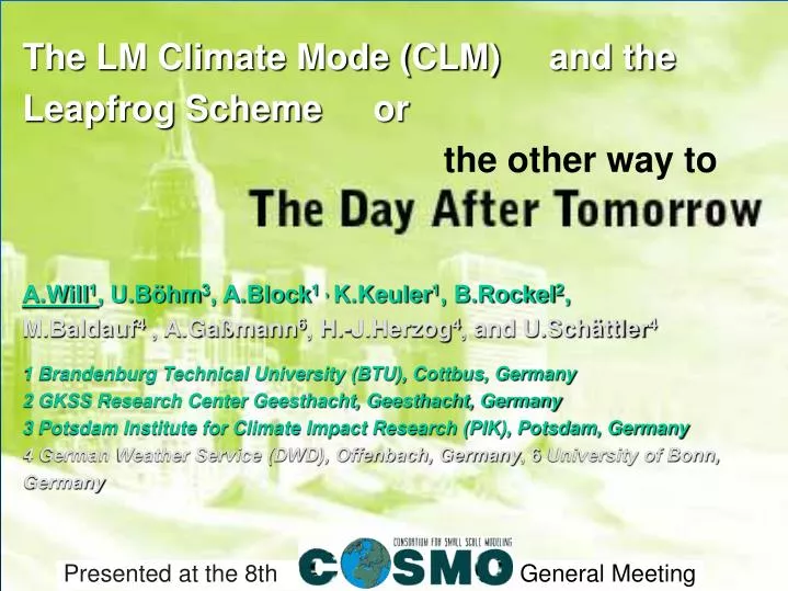
The LM Climate Mode (CLM)and the Leapfrog Scheme or the other way toA.Will1, U.Böhm3, A.Block1 , K.Keuler1, B.Rockel2,M.Baldauf4 , A.Gaßmann6, H.-J.Herzog4, and U.Schättler41 Brandenburg Technical University (BTU), Cottbus, Germany2 GKSS Research Center Geesthacht, Geesthacht, Germany3 Potsdam Institute for Climate Impact Research (PIK), Potsdam, Germany4 German Weather Service (DWD), Offenbach, Germany, 6 University of Bonn, Germany Presented at the 8th General Meeting
Model run configuration: CLM_2.4.8 -> www.clm-community.eu and LM_3.19 Model domain: EURope (193 x 217) Extended EURope (256x271) LME Data: ERA40 GME ECHAM5+OPYC Dx = 18km Dt := 90 s for leapfrog • TERRA_MLβ • 10 Layers • z_1=1cm, z_10=11.5m • Dts = 30 s
Developed by the CLM-Community in cooperation with the German weather service TOT_PREC + ∆ v, mean July 60, ECHAM5 DT=90, DX=0.165 Film: TOT_PREC+PP
Variation of Configuration CFL: V < 160 km/h for DT=90
Developed by the CLM-Community in cooperation with the German weather service TOT_PREC + ∆ v, mean July 60, ECHAM5 EXT, DX=0.44 DT=90, DX=0.165
Developed by the CLM-Community in cooperation with the German weather service TOT_PREC + ∆ v, mean July 60, ECHAM5 DX=0.165 nested in DX=0.=0.44 DT=90, DX=0.165
Developed by the CLM-Community in cooperation with the German weather service 000 [mm] Climate Mode, mean July 79-94, ERA15 climate modeModel Results Outlook
Dependence on the time step: CLM_2.4.8, DX=0.165, KON≈LME Shower
T(l,t) central Spain 7/60 DT=90 DT=75 DT=60 DTS=30 DTS=10 DTS=30 DTS=18.75 DTS=10 DTS=30 DTS=10 300 K 280 K 220 K
Overview: Leapfrog, CLM_2.4.8, DX=0.165, KON≈LME Shower ,,The day after tomorrow‘‘ Shower
Model Physics LM 3.19, DX=0.165, LME-Region, DTS=30s Shower ??? Simulation series calculated by Ulrich Schättler
Joining Skills of weather forecast and (regional) climate modelling Weather Forecast • Detailed analysis of weather phenomena in a nonhydrostatic model • Extended model tests in the operational wether forecast • Systematic development of physical parameterizations • Further development of numerical schemes • Climate Modelling • Separation of model physics, initial and boundary conditions and data assimilation • Detection of potential short-comings of LM clearly visible in long-term integrations. • Assessment of climatologically relevant components (hydrological cycle, soil, conservation principles). • Further development of the climate mode: “open” boundary conditions, new modules for aerosols, chemistry, biosphere and SST-dynamics , globally conserving and dispersion free numerical schemes for improved operational weather forecast and regional climate prediction with the hybrid LM/CLM Thank you for attention !
2002 6.2003 3.2004 12.2005 10.2006
Climate mode Forecast mode Integration time 100y and more (from restart) 78h Dependence on initial values no / weak after spin up strong Nudging of observations possible yes vegetation, CO2 etc., SSTs prescribed constant Conservation principles high sensitivity hardly detectable The climate and the forecast mode Statistics • Dependence on initial conditions no yes • Dependence on boundary condit. Yes yes • Dependence on observations weak strong