Download
1 / 74
740 likes | 777 Views
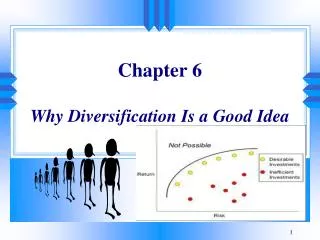
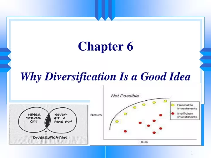
Chapter 6 Why Diversification Is a Good Idea. Lessons from Evans and Archer. Introduction Methodology Results Implications Words of caution. Introduction. Evans and Archer’s 1968 Journal of Finance article Very consequential research regarding portfolio construction

E N D
Lessons from Evans and Archer • Introduction • Methodology • Results • Implications • Words of caution
Introduction • Evans and Archer’s 1968 Journal of Finance article • Very consequential research regarding portfolio construction • Shows how naïve diversification reduces the dispersion of returns in a stock portfolio • Naïve diversification refers to the selection of portfolio components randomly
Methodology • Used computer simulations: • Measured the average variance of portfolios of different sizes, up to portfolios with dozens of components • Purpose was to investigate the effects of portfolio size on portfolio risk when securities are randomly selected
Results • Definitions • General results • Strength in numbers • Biggest benefits come first • Superfluous diversification
Definitions • Systematic risk is the risk that remains after no further diversification benefits can be achieved • Unsystematic risk is the part of total risk that is unrelated to overall market movements and can be diversified • Research indicates up to 75 percent of total risk is diversifiable
Definitions (cont’d) • Investors are rewarded only for systematic risk • Rational investors should always diversify • Explains why beta (a measure of systematic risk) is important • Securities are priced on the basis of their beta coefficients
General Results Portfolio Variance Number of Securities
Strength in Numbers • Portfolio variance (total risk) declines as the number of securities included in the portfolio increases • On average, a randomly selected ten-security portfolio will have less risk than a randomly selected three-security portfolio • Risk-averse investors should always diversify to eliminate as much risk as possible
Biggest Benefits Come First • Increasing the number of portfolio components provides diminishing benefits as the number of components increases • Adding a security to a one-security portfolio provides substantial risk reduction • Adding a security to a twenty-security portfolio provides only modest additional benefits
Superfluous Diversification • Superfluous diversification refers to the addition of unnecessary components to an already well-diversified portfolio • Deals with the diminishing marginal benefits of additional portfolio components • The benefits of additional diversification in large portfolio may be outweighed by the transaction costs
Implications • Very effective diversification occurs when the investor owns only a small fraction of the total number of available securities • Institutional investors may not be able to avoid superfluous diversification due to the dollar size of their portfolios • Mutual funds are prohibited from holding more than 5 percent of a firm’s equity shares
Implications (cont’d) • Owning all possible securities would require high commission costs • It is difficult to follow every stock
Words of Caution • Selecting securities at random usually gives good diversification, but not always • Industry effects may prevent proper diversification • Although naïve diversification reduces risk, it can also reduce return • Unlike Markowitz’s efficient diversification
Markowitz’s Contribution • Harry Markowitz’s “Portfolio Selection” Journal of Finance article (1952) set the stage for modern portfolio theory • The first major publication indicating the important of security return correlation in the construction of stock portfolios • Markowitz showed that for a given level of expected return and for a given security universe, knowledge of the covariance and correlation matrices are required
Quadratic Programming • The Markowitz algorithm is an application of quadratic programming • The objective function involves portfolio variance • Quadratic programming is very similar to linear programming
Portfolio Programming in a Nutshell • Various portfolio combinations may result in a given return • The investor wants to choose the portfolio combination that provides the least amount of variance
Concept of Dominance • Dominance is a situation in which investors universally prefer one alternative over another • All rational investors will clearly prefer one alternative
Concept of Dominance (cont’d) • A portfolio dominates all others if: • For its level of expected return, there is no other portfolio with less risk • For its level of risk, there is no other portfolio with a higher expected return
Concept of Dominance (cont’d) Example (cont’d) In the previous example, the B/C combination dominates the A/C combination: B/C combination dominates A/C Expected Return Risk
Terminology • Security Universe • Efficient frontier • Capital market line and the market portfolio • Security market line • Expansion of the SML to four quadrants • Corner portfolio
Security Universe • The security universe is the collection of all possible investments • For some institutions, only certain investments may be eligible • E.g., the manager of a small cap stock mutual fund would not include large cap stocks
Efficient Frontier • Construct a risk/return plot of all possible portfolios • Those portfolios that are not dominated constitute the efficient frontier
Efficient Frontier (cont’d) Expected Return 100% investment in security with highest E(R) No points plot above the line Points below the efficient frontier are dominated All portfolios on the line are efficient 100% investment in minimum variance portfolio Standard Deviation
Efficient Frontier (cont’d) When a risk-free investment is available, the shape of the efficient frontier changes • The expected return and variance of a risk-free rate/stock return combination are simply a weighted average of the two expected returns and variance The risk-free rate has a variance of zero
Efficient Frontier (cont’d) Expected Return C B Rf A Standard Deviation
Efficient Frontier (cont’d) • The efficient frontier with a risk-free rate: • Extends from the risk-free rate to point B • The line is tangent to the risky securities efficient frontier • Follows the curve from point B to point C
Theorem For any constant Rf on the returns axis, the weights of the tangency portfolio B are:
What is the zero-beta portfolio? • The zero beta portfolio P0 is the portfolio determined by the intersection of the frontier with a horizontal line originating from the constant Rf selected. • Property: whatever Rf we choose, we always have Cov(B,P0)=0 (Notice, however, that the location of B and P0 will depend on the value selected for Rf)
Note that the last proposition is true even if the risk-free rate (i.e. a riskless security) doesn’t exist in the economy. • The way the tangency portfolio B was determined also remains valid even if there is no riskless rate in the economy. • All one has to do is replace Rf by a chosen constant c. The mathematics of the last propositions will remain valid.
Fisher Black zero beta CAPM (1972) • For a chosen constant c on the vertical axis of returns, the tangency portfolio B can be computed, and for ANY portfolio x we have a linear relationship if we regress the returns of x on the returns of B: • Moreover, c is the expected rate of return of a portfolio P0 whose covariance with B is zero.
Fisher Black zero beta CAPM (Cont’d) • The name “zero beta” stems from the fact that the covariance between P0 and B is zero, since a zero covariance implies that the beta of P0 with respect to B is zero too. • If a riskless asset DOES exist in the economy, however, we can replace the constant c in Black’s zero beta CAPM by Rf and the portfolio B is the market portfolio.
Capital Market Line and the Market Portfolio • The tangent line passing from the risk-free rate through point B is the capital market line (CML) • When the security universe includes all possible investments, point B is the market portfolio • It contains every risky assets in the proportion of its market value to the aggregate market value of all assets • It is the only risky assets risk-averse investors will hold
Capital Market Line and the Market Portfolio (cont’d) • Implication for investors: • Regardless of the level of risk-aversion, all investors should hold only two securities: • The market portfolio • The risk-free rate • Conservative investors will choose a point near the lower left of the CML • Growth-oriented investors will stay near the market portfolio
Capital Market Line and the Market Portfolio (cont’d) • Any risky portfolio that is partially invested in the risk-free asset is a lending portfolio • Investors can achieve portfolio returns greater than the market portfolio by constructing a borrowing portfolio
Capital Market Line and the Market Portfolio (cont’d) Expected Return C B Rf A Standard Deviation
Security Market Line • The graphical relationship between expected return and beta is the security market line (SML) • The slope of the SML is the market price of risk • The slope of the SML changes periodically as the risk-free rate and the market’s expected return change
Security Market Line (cont’d) Expected Return E(R) Market Portfolio Rf 1.0 Beta
Notice that we obtained very poor results. The R-squared is only 27.93% ! • However, the math of the CAPM is undoubtedly true. • How then can CAPM fail in the real world? • Possible explanations are that true asset returns distributions are unobservable, individuals have non-homogenous expectations, the market portfolio is unobservable, the riskless rate is ambiguous, markets are not friction-free.
We obtained a perfect 100% R-squared this time ! • The reason is that when portfolio returns are regressed on their betas with respect to an efficient portfolio, an exact linear relationship holds.
Expansion of the SML to Four Quadrants • There are securities with negative betas and negative expected returns • A reason for purchasing these securities is their risk-reduction potential • E.g., buy car insurance without expecting an accident • E.g., buy fire insurance without expecting a fire
Security Market Line (cont’d) Expected Return Securities with Negative Expected Returns Beta
Diversification and Beta • Beta measures systematic risk • Diversification does not mean to reduce beta • Investors differ in the extent to which they will take risk, so they choose securities with different betas • E.g., an aggressive investor could choose a portfolio with a beta of 2.0 • E.g., a conservative investor could choose a portfolio with a beta of 0.5
Capital Asset Pricing Model • Introduction • Systematic and unsystematic risk • Fundamental risk/return relationship revisited
Introduction • The Capital Asset Pricing Model (CAPM) is a theoretical description of the way in which the market prices investment assets • The CAPM is a positive theory