Download
1 / 52
520 likes | 522 Views
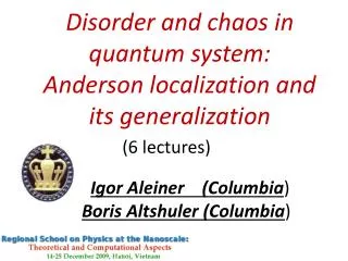
Disorder and chaos in quantum systems II. Lecture 2. Boris Altshuler Physics Department, Columbia University. Previous Lecture:. Anderson Localization as Metal-Insulator Transition Anderson model. Localized and extended states. Mobility edges.

E N D
Disorder and chaos in quantum systems II. Lecture 2. Boris AltshulerPhysics Department, Columbia University
Previous Lecture: Anderson Localization as Metal-Insulator Transition Anderson model. Localized and extended states. Mobility edges. 2. Spectral Statistics and Localization. Poisson versus Wigner-Dyson. Anderson transition as a transition between different types of spectra. Thouless conductance P(s) Conductance g s
Lecture2. 1. Quantum Chaos, Integrabilityand Localization
P(s) Particular nucleus 166Er s P(s) Spectra of several nuclei combined (after spacing) rescaling by the mean level N. Bohr, Nature 137 (1936) 344.
? Q: Why the random matrix theory (RMT) works so well for nuclear spectra These are systems with a large number of degrees of freedom, and therefore the “complexity” is high Original answer: Later it became clear that there exist very “simple” systems with as many as 2 degrees of freedom (d=2), which demonstrate RMT - like spectral statistics
Classical (h =0) Dynamical Systems withd degrees of freedom dintegrals of motion The variables can be separated and the problem reduces todone-dimensional problems Integrable Systems Examples 1. A ball inside rectangular billiard;d=2 • Vertical motion can be separatedfrom the horizontal one • Vertical and horizontal components of the momentum, are both integrals of motion 2. Circular billiard;d=2 • Radial motion can be separatedfrom the angular one • Angular momentum and energy are the integrals of motion
Classical Dynamical Systems with d degrees of freedom Integrable Systems The variables can be separated [done-dimensional problems [dintegrals of motion Rectangular and circular billiard, Kepler problem, . . . , 1d Hubbard model and other exactly solvable models, . . The variables can not be separated [there is only one integral of motion - energy Chaotic Systems Examples B Kepler problem in magnetic field Stadium Sinai billiard
Nonlinearities • Exponential dependence on the original conditions (Lyapunov exponents) • Ergodicity Classical Chaos h =0 Quantum description of any System with a finite number of the degrees of freedom is a linear problem – Shrodinger equation Q:What does it mean Quantum Chaos?
Bohigas – Giannoni – Schmit conjecture Chaotic classical analog Wigner- Dyson spectral statistics No quantum numbers except energy
Quantum Classical ? Integrable Poisson ? Wigner-Dyson Chaotic
Lecture1. 2. Localization beyond real space
Kolmogorov – Arnold – Moser (KAM) theory A.N. Kolmogorov, Dokl. Akad. Nauk SSSR, 1954. Proc. 1954 Int. Congress of Mathematics, North-Holland, 1957 Integrable classical Hamiltonian , d>1: Separation of variables: d sets of action-angle variables Andrey Kolmogorov Vladimir Arnold Jurgen Moser
Kolmogorov – Arnold – Moser (KAM) theory A.N. Kolmogorov, Dokl. Akad. Nauk SSSR, 1954. Proc. 1954 Int. Congress of Mathematics, North-Holland, 1957 Integrable classical Hamiltonian , d>1: Separation of variables: d sets of action-angle variables Quasiperiodic motion: set of the frequencies, which are in general incommensurate. Actions are integrals of motion Andrey Kolmogorov …=> Vladimir Arnold tori Jurgen Moser
Integrable dynamics: Each classical trajectory is quasiperiodic and confined to a particular torus, which is determined by a set of the integrals of motion For d>1 each torus has measure zero on the energy shell !
Kolmogorov – Arnold – Moser (KAM) theory Integrable classical Hamiltonian , d>1: A.N. Kolmogorov, Dokl. Akad. Nauk SSSR, 1954. Proc. 1954 Int. Congress of Mathematics, North-Holland, 1957 Separation of variables: d sets of action-angle variables Quasiperiodic motion: set of the frequencies, which are in general incommensurate Actions are integrals of motion …=> ? Q: Will an arbitrary weak perturbation of the integrable Hamiltonian destroy the tori and make the motion ergodic (when each point at the energy shell will be reached sooner or later) Andrey Kolmogorov A: Most of the tori survive weak and smooth enough perturbations KAM theorem Vladimir Arnold Jurgen Moser
KAM theorem: Most of the tori survive weak and smooth enough perturbations ? Each point in the space of the integrals of motion corresponds to a torus and vice versa Finite motion. Localization in the space of the integrals of motion
KAM theorem: Most of the tori survive weak and smooth enough perturbations Energy shell
Consider an integrable system. Each state is characterized by a set of quantum numbers. It can be viewed as a point in the space of quantum numbers. The whole set of the states forms a lattice in this space. A perturbationthat violates the integrability provides matrix elements of the hopping between different sites (Anderson model!?) Weak enough hopping: Localization - Poisson Strong hopping: transition to Wigner-Dyson
Sinai billiard Square billiard Disordered localized Disordered extended Localized real space Localized momentum space extended
Extended states: Level repulsion, anticrossings, Wigner-Dyson spectral statistics Localized states: Poisson spectral statistics Invariant (basis independent) definition
Chaotic Integrable All chaotic systems resemble each other. Sinai billiard Square billiard All integrable systems are integrable in their own way Disordered extended Disordered localized
Consider a finite system of quantum particles, e.g., fermions. Let the one-particle spectra be chaotic (Wigner-Dyson). What is the statistics of the many-body spectra? ? Q: • The particles do not interact with each other. • Poisson: • individual energies are conserving quantum numbers. • b. The particles do interact. ????
Lecture 2. 3. Many-Body excitation in finite systems
Decay of a quasiparticle with an energy e in Landau Fermi liquid e Fermi Sea
Quasiparticle decay rate at T = 0in a clean Fermi Liquid. I. d=3 Fermi Sea • Reasons: • At small the energy transfer, w , is small and the integration over and w gives the factor 2. ………………………………………………………………… • The momentum transfer, q , is large and thus the scattering probability at given and w does not depend on , w or
Quasiparticle decay rate at T = 0in a clean Fermi Liquid. II. Low dimensions e Small moments transfer, q , become important at low dimensions because the scattering probability is proportional to the squared time of the interaction, (qvF. )-2 vF 1/q
Quasiparticle decay rate at T = 0in a clean Fermi Liquid. Quasiparticle decayrate atT = 0in a cleanFermi Liquid. Fermi Sea Conclusions: 1. For d=3,2from it follows that , i.e., that the qusiparticles are well determined and the Fermi-liquid approach is applicable. 2. For d=1is of the order of , i.e., that the Fermi-liquid approach is not valid for 1d systems of interacting fermions. Luttinger liquids
Decay of a quasiparticle with an energy e in Landau Fermi liquid Quantum dot – zero-dimensional case ? e e-w e1+w Fermi Sea e1
Decay of a quasiparticle with an energy e in Landau Fermi liquid Quantum dot – zero-dimensional case ? e Decay rate of a quasiparticle with energye e-w (U.Sivan, Y.Imry & A.Aronov,1994 ) Fermi Golden rule: e1+w Fermi Sea e1 Mean level spacing Thouless energy
Decay rate of a quasiparticle with energye in 0d. (U.Sivan, Y.Imry & A.Aronov,1994 ) Fermi Golden rule: Recall: Thouless conductance Mean level spacing Thouless energy Zero dimensional system Def: One particle states are extended all over the system
Decay rate of a quasiparticle with energye in 0d. Problem: zero-dimensional case e e-w one-particle spectrum is discrete e1+w equation e1+e2= e’1+ e’2 can not be satisfied exactly Fermi Sea e1 Recall:in the Anderson model the site-to-site hopping does not conserve the energy
Decay rate of a quasiparticle with energye in 0d. e e-w e’+ w e’ Offdiagonal matrix element
Chaos in Nuclei – Delocalization? 1 2 3 4 5 6 Delocalization in Fock space e generations e’ Can be mapped (approximately) to the problem of localization on Cayley tree . . . . e1’ 1 2 3 4 5 Fermi Sea e1
Conventional Anderson Model • one particle, • one level per site, • onsite disorder • nearest neighbor hoping labels sites Basis: Hamiltonian:
0d system; no interactions ea many (N ) particles no interaction: Individual energies and thus occupation numbers are conserved eb eg Nconservation laws “integrable system” ed integrable system
0d system with interactions ea Basis: eb occupation numbers labels levels eg Hamiltonian: ed
Conventional Anderson Model Many body Anderson-like Model Basis: Basis: occupation numbers labels levels labels sites “nearest neighbors”:
Isolated quantum dot – 0d system of fermions Exact many-body states: Ground state, excited states Exact means that the imaginary part of the energy is zero! Quasiparticle excitations: Finite decay rate Q: ? What is the connection
S gate QD source drain D current No e-e interactions – resonance tunneling
S gate QD source drain D current g No e-e interactions – resonance tunneling Mean level spacing d1 VSD
S gate QD source drain D current g The interaction leads to additional peaks – many body excitations No e-e interactions – resonance tunneling VSD
S S D D Resonance tunneling Peaks Inelastic cotunneling Additional peak
S gate QD source drain S current g The interaction leads to additional peaks – many body excitations VSD
S gate QD source drain D current g Landau quasiparticle with the widthgSIA NE Ergodic - WD loc VSD
Landau quasiparticle with the widthgSIA NE Ergodic - WD loc VSD extended Localized - finite # of the satelites Extended - infinite # of the satelites (for finite e the number of the satelites is always finite) Ergodic – nonergodic crossover!
Anderson Model on a Cayley tree I, W K – branching number Resonance at every generation Sparse resonances
Definition: We will call a quantum state ergodic if it occupies the number of sites on the Anderson lattice, which is proportional to the total number of sites : ergodic nonergodic Localized states are obviously not ergodic: ? Q: Is each of the extended state ergodic A: In 3D probably yes For d>4 most likely no