Download
1 / 20
290 likes | 1.88k Views
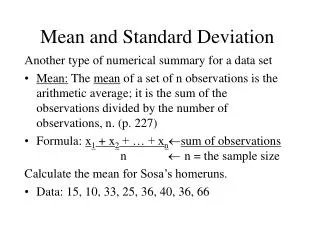
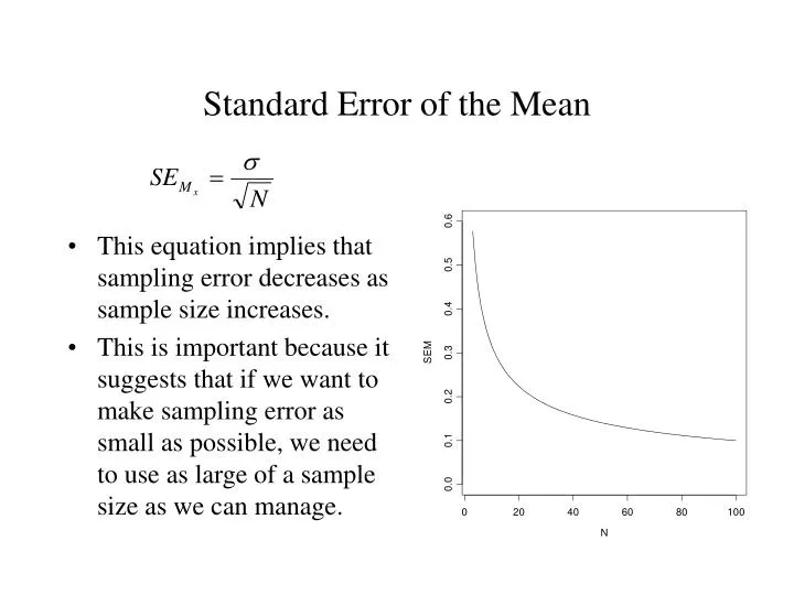
Standard Error of the Mean. This equation implies that sampling error decreases as sample size increases. This is important because it suggests that if we want to make sampling error as small as possible, we need to use as large of a sample size as we can manage. Standard Error of the Mean.

E N D
Standard Error of the Mean • This equation implies that sampling error decreases as sample size increases. • This is important because it suggests that if we want to make sampling error as small as possible, we need to use as large of a sample size as we can manage.
Standard Error of the Mean • The SE provides a useful way to quantify sampling error. • It is useful because it allows us to represent the amount of sampling error associated with our sampling process—how much error we can expect on average. • Example: If we are sampling (N = 7) from a population in which mu is 3.6 and sigma is 1.36, then the SE will be approximately .50. We expect, on average, observed sample means of 3.6, but, when we’re wrong, we expect to be off by about .5 points, on average.
Confidence Intervals • Technically, the SE is also called a 68% confidence interval. • Recall that the distribution of sampling errors resembles a normal curve. We learned earlier, in the days of z-scores, that 68% of scores fall between –1 and + 1 standard deviations from the mean. • By extension, then, we can say that 68% of sample means will fall between – 1 SE and + 1 SE.
The area under a normal curve 0.4 Mu = 3.6 SE = .5 0.3 0.2 34% 34% 0.1 14% 14% 2% 2% 0.0 1.6 2.1 2.6 3.1 3.6 4.1 4.6 5.1 5.6 Sample Mean
68% Confidence Intervals • Thus, in forward inference, a 68% confidence interval marks the bounds within which 68% of the sample means will fall, given certain facts about the population and the sampling process. • lower bound of the CI: – SE • upper bound of the CI: + SE
95% Confidence Intervals • Sometimes people use 95% confidence intervals. • lower bound: – 1.96 SE • upper bound: + 1.96 SE
lower bound: 3.6 – 1.96 .5 = 2.62 upper bound: 3.6 + 1.96 .5 = 4.58 Thus, the 95% confidence interval ranges from 2.62 to 4.58. Under the sampling conditions described, 95% of the time we will observe sample means between 2.62 and 4.58. n = 7 mean of sample means = 3.6 SD of sample means = .5
Backward Inference • What we’ve been describing is a variety of inferential statistics that I call “forward inference.” • That is, given certain facts of the population and sampling conditions, we can make inferences about the statistical properties of samples that might be observed.
Backward Inference • In many applied research situations, we don’t know the facts of the population. • We know the sampling conditions (e.g., random sample of size 100) and the facts of the sample (i.e., the sample mean and standard deviation). • How do we make inference about the properties of the population from this information?
Backwards Inference • Backwards inference is based on a critical assumption: That the a priori likelihood of all possible population means are equivalent. • This assumption tends to be ignored in undergraduate statistics textbooks (including yours) and in practice. We’ll discuss this problem in more detail in a few weeks (Bayesian statistics), but, for now, let’s explore backwards inference as it typically applied.
Example • Let’s begin with a situation in which we take a random sample of 5 people from a population (1, 2, 3, 4, 4, 5, 4, 6, 3, 4, mu = 3.6, sigma = 1.36), compute a sample mean, and, based on this, try to infer the mean for the population from which our sample was drawn. • We get the following sample scores: 4, 4, 6, 4, 3 (M = 4.2, SD = .98) • Important assumption: Prior to observing our sample mean, all possible population means are equally likely. In other words, a mu of 3.6 is just as likely as a mu of 4.2.
Means: Backward Inference • Under this assumption, we can simply flip or reverse the forward inferential logic used earlier. • The “best guess” for the population mean is the sample mean (4.2) because we know that the sample mean is unbiased. If the population mean is the expected value of a sample mean in forward inference (i.e., the best guess as to what sample mean we might observe), then the sample mean is the best guess about the population mean in backward inference.
Variances: Backward Inference • For variances, we can again flip the forward inferential logic we used earlier. • Recall that the population variance is typically a bit larger than the expected sample variance. Hence, the variance we observe in our sample is a little too small to be a good estimate of the population variance. • We can correct it by making it a little bit larger by dividing by N – 1 instead of N. (This is exactly how much we need to correct the sample variance to make it an unbiased estimate of the population variance.) .98 (unadjusted sample mean) vs. (4.8/4) = 1.2 (adjusted sample mean)
Confidence Intervals: Backward Inference • Similarly, we can reconceptualize confidence intervals within the framework of backwards inference. • In our example with forward inference, we said that, under certain sampling conditions, samples drawn from our population will have means that fall between 3.1 and 4.1 95% of the time.
Confidence Intervals: Backwards Inference • In backwards inference, we say that this method of constructing intervals will capture the population mean 95% of the time.
lower bound: Mx – 1.96 SE • upper bound: Mx + 1.96 SE • (We have to use an estimate the population standard deviation because we do not know it. Recall that the sample SD is biased, so we have to used the corrected, unbiased formula to estimate it correctly.)
lower bound: 4.2 – 1.96 .53 = 3.16 • upper bound: 4.2 + 1.96 .53 = 5.23 • Thus, we say that there is a 95% chance that the population mean falls between these two values: 3.16 and 5.23.
samples In forward inference, we can say that this method of constructing intervals will capture the observed sample mean 95% of the time. In backwards inference, we can say that this method of constructing intervals will capture the population mean 95% of the time.
Sometimes in backwards inference the CI is interpreted as implying that there is a 95% chance that the population mean falls within this interval. • This is logic is problematic for reasons we’ll discuss later in the course. But, for now, if we assume that there is no particular value of the population mean that is more likely prior to our study, then this logic is sensible.