Download
1 / 50
500 likes | 686 Views
The Fifth SIAM workshop on Combinatorial Scientific Computing. Darmstadt, May 19-21 2011. Graph Expansion and Communication Costs of Fast Matrix Multiplication. Oded Schwartz 1. Joint work with: Grey Ballard 1 , James Demmel 1 , Olga Holtz 1,2 1. UC-Berkeley 2. TU-Berlin.

E N D
The Fifth SIAM workshop onCombinatorial Scientific Computing Darmstadt, May 19-21 2011 Graph Expansion andCommunication Costs of Fast Matrix Multiplication Oded Schwartz1 Joint work with: Grey Ballard1, James Demmel1, Olga Holtz1,2 1. UC-Berkeley 2. TU-Berlin Best PaperAward
Results by: • Grey Ballard, UCB • AydinBuluc, LBL • Erin Carson, UCB • James Demmel, UCB • Jack Dongarra, UTK • IoanaDumitriu, U. Washington • Laura Grigori, INRIA • Ming Gu, UCB Math • Mark Hoemmen, Sandia NL • Olga Holtz, UCB Math & TU Berlin • Nicholas Knight, UCB • JulienLangou, U. Colorado Denver • EranRom, IBM Tel-Aviv • Edgar Solomonik, UCB • Hua Xiang, INRIA Many others…
Motivation Two kinds of costs: Arithmetic (FLOPs) Communication: moving data between levels of a memory hierarchy (sequential case) over a network connecting processors (parallel case) Communication-avoiding algorithm: Save time, save energy. CPU Cache CPU RAM CPU RAM M1 M2 RAM M3 CPU RAM CPU RAM Mk = From cloud computing to mobile devices. IT: 3% of US energy Parallel Sequential Hierarchy
Motivation: expected bottleneck CPU Cache CPU RAM CPU RAM M1 M2 RAM M3 CPU RAM CPU RAM Mk = Parallel Sequential Hierarchy
Outline Algorithms with “flavor” of 3 nested loops • Lower bounds: Sequential, Hierarchy, Parallel. • Algorithms: Sequential, Parallel 2D, Parallel 2.5D Strassen-like algorithms • Lower bounds: Sequential, Hierarchy, Parallel. • Algorithms: Sequential, Parallel 2D, Parallel 2.5D • [Ballard, Demmel, Holtz, S. 2009],[Ballard, Demmel, Holtz, S. 2011a] extending[Hong & Kung 81], [Irony,Toledo,Tiskin 04] • Many contributions, mostly new • [Ballard, Demmel, Holtz, S. 2011b] • [Ballard, Demmel, Holtz, Rom, S. 2011]
Lower bounds: for algorithms with “flavor” of 3 nested loops Matrix Multiplication [Hong & Kung 81] Sequential [Irony,Toledo,Tiskin 04] Sequential and parallel
Lower bounds: for algorithms with “flavor” of 3 nested loops [Ballard, Demmel, Holtz, S. 2009],[Ballard, Demmel, Holtz, S. 2011a] Following [Irony,Toledo,Tiskin 04] BLAS, LU, Cholesky, LDLT, and QR factorizations, eigenvalues and singular values, i.e., essentially all direct methods of linear algebra. Dense or sparse matrices In sparse cases: bandwidth is a function NNZ. Bandwidth and latency. Sequential, hierarchical, and parallel – distributed and shared memory models. Compositions of linear algebra operations. Certain graph optimization problems [Demmel, Pearson, Poloni, Van Loan, 11] Tensor contraction
Do conventional dense algorithms as implemented in • LAPACK and ScaLAPACK attain these bounds? • Mostly not. • Are there other algorithms that do? • Mostly yes.
Outline Algorithms with “flavor” of 3 nested loops • Lower bounds: Sequential, Hierarchy, Parallel. • Algorithms: Sequential, Parallel 2D, Parallel 2.5D Strassen-like algorithms • Lower bounds: Sequential, Hierarchy, Parallel. • Algorithms: Sequential, Parallel 2D, Parallel 2.5D • [Ballard, Demmel, Holtz, S. 2009],[Ballard, Demmel, Holtz, S. 2011a] extending[Hong & Kung 81], [Irony,Toledo,Tiskin 04] • Many contributions, mostly new • [Ballard, Demmel, Holtz, S. 2011b] • [Ballard, Demmel, Holtz, Rom, S. 2011]
Dense 2D parallel algorithms memory per processor = O(n2 / P) • Assume nxn matrices on P processors, memory per processor = O(n2 / P) • ScaLAPACK assumes best block size b chosen • Many references (see reports), Blueare new • Recall lower bounds: • #words_moved = ( n2 / P1/2 ) and #messages = ( P1/2 ) Can these be improved?
New 2.5D parallel algorithms: Matrix multiplication and LU decomposition c ∙ 3n2 = M∙P cis the memory multiplicity factor (c may be bounded by P): [Solomonik, Demmel, 2011]: Distinguished paper EuroPar’11c1/2 times fewer words communicated than [Cannon 69]. [Irony,Toledo,Tiskin 04], [Ballard, Demmel, Holtz, S. 2011a]:This is as good as it gets.
Motivation: a few example speedups,Measured and Predicted [Demmel, Ballard, Hoemmen, Grigori, Langou, Dongarra, Anderson 10] [Anderson, Ballard, Demmel Keutzer 10] [Bhatele, Demmel, Solomonik 11] Measured: Parallel TSQR • Intel Clovertown • Up to 8x speedup (8 core, dual socket, 10M x 10) • Pentium III cluster, Dolphin Interconnect, MPICH • Up to 6.7x speedup (16 procs, 100K x 200) • BlueGene/L • Up to 4x speedup (32 procs, 1M x 50) • Tesla C 2050 / Fermi • Up to 13x (110,592 x 100) Predicted: Parallel 2.5D LU • Exascale • Up to 4.5x speedup (218 nodes, 222x222)
Beyond 3-nested loops How about the communication costs of algorithms that have a more complex structure?
Outline Algorithms with “flavor” of 3 nested loops • Lower bounds: Sequential, Hierarchy, Parallel. • Algorithms: Sequential, Parallel 2D, Parallel 2.5D Strassen-like algorithms • Lower bounds: Sequential, Hierarchy, Parallel. • Algorithms: Sequential, Parallel 2D, Parallel 2.5D • [Ballard, Demmel, Holtz, S. 2009],[Ballard, Demmel, Holtz, S. 2011a] extending[Hong & Kung 81], [Irony,Toledo,Tiskin 04] • Many contributions, mostly new • [Ballard, Demmel, Holtz, S. 2011b] • [Ballard, Demmel, Holtz, Rom, S. 2011]
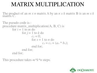
[Strassen 69] Compute 2 x 2 matrix multiplication using only 7 multiplications (instead of 8). Apply recursively (block-wise) M1 = (A11 + A22) (B11 + B22) M2 = (A21 + A22) B11 M3 = A11 (B12 - B22) M4 = A22 (B21 - B11) M5 = (A11+ A12) B22 M6 = (A21 - A11) (B11 + B12) M7 = (A12 - A22) (B21 + B22) C11 = M1 + M4 - M5 + M7 C12 = M3 + M5 C21 = M2 + M4 C22 = M1 - M2 + M3 + M6 Recall: Strassen’s Fast Matrix Multiplication A11 A12 B11 B12 n/2 = A21 A22 B21 B22 n/2 C11 C12 C21 C22 T(n) = 7T(n/2) + O(n2) T(n) = (nlog27)
Strassen-like algorithms Compute n0 x n0 matrix multiplication using only n00 multiplications (instead of n03). Apply recursively (block-wise) 0 2.81 [Strassen 69] works fast in practice. 2.79 [Pan 78] 2.78 [Bini 79] 2.55 [Schönhage 81] 2.50 [Pan Romani,CoppersmithWinograd 84] 2.48 [Strassen 87] 2.38 [Coppersmith Winograd 90] 2.38 [Cohn Kleinberg SzegedyUmans 05] Group-theoretic approach n/n0 = T(n) = n00T(n/n0) + O(n2) T(n) = (n0)
Outline Algorithms with “flavor” of 3 nested loops • Lower bounds: Sequential, Hierarchy, Parallel. • Algorithms: Sequential, Parallel 2D, Parallel 2.5D Strassen-like algorithms • Lower bounds: Sequential, Hierarchy, Parallel. • Algorithms: Sequential, Parallel 2D, Parallel 2.5D • [Ballard, Demmel, Holtz, S. 2009],[Ballard, Demmel, Holtz, S. 2011a] extending[Hong & Kung 81], [Irony,Toledo,Tiskin 04] • Many contributions, mostly new • [Ballard, Demmel, Holtz, S. 2011b] • [Ballard, Demmel, Holtz, Rom, S. 2011]
New lower bound for Strassen’s fast matrix multiplication [Ballard, Demmel, Holtz, S. 2011b]: The Communication bandwidth lower bound is For Strassen’s: Strassen-like: Recall for cubic: 0 log2 8 log2 7 The parallel lower bounds applies to2D: M = (n2/P) 2.5D: M = (c∙n2/P)
For sequential? hierarchy? • Yes, existing implementation do! • For parallel 2D? parallel 2.5D? • Yes: new algorithms.
Outline Algorithms with “flavor” of 3 nested loops • Lower bounds: Sequential, Hierarchy, Parallel. • Algorithms: Sequential, Parallel 2D, Parallel 2.5D Strassen-like algorithms • Lower bounds: Sequential, Hierarchy, Parallel. • Algorithms: Sequential, Parallel 2D, Parallel 2.5D • [Ballard, Demmel, Holtz, S. 2009],[Ballard, Demmel, Holtz, S. 2011a] extending[Hong & Kung 81], [Irony,Toledo,Tiskin 04] • Many contributions, mostly new • [Ballard, Demmel, Holtz, S. 2011b] • [Ballard, Demmel, Holtz, Rom, S. 2011]
Sequential and new 2D and 2.5D parallel Strassen-like algorithms Sequential and Hierarchy cases: Attained by the natural recursive implementation. Also: LU, QR,… (Black-box use of fast matrix multiplication) [Ballard, Demmel, Holtz, S., Rom 2011]: New 2D parallel Strassen-like algorithm.Attains the lower bound. New 2.5D parallel Strassen-like algorithm.c 0 /2-1 parallel communication speedup over 2D implementation (c ∙ 3n2 = M∙P) [Ballard, Demmel, Holtz, S. 2011b]:This is as good as it gets.
Outline Algorithms with “flavor” of 3 nested loops • Lower bounds: Sequential, Hierarchy, Parallel. • Algorithms: Sequential, Parallel 2D, Parallel 2.5D Strassen-like algorithms • Lower bounds: Sequential, Hierarchy, Parallel. • Algorithms: Sequential, Parallel 2D, Parallel 2.5D • [Ballard, Demmel, Holtz, S. 2009],[Ballard, Demmel, Holtz, S. 2011a] extending[Hong & Kung 81], [Irony,Toledo,Tiskin 04] • Many contributions, mostly new • [Ballard, Demmel, Holtz, S. 2011b] • [Ballard, Demmel, Holtz, Rom, S. 2011]
Communication Lower Bounds Approaches: Reduction [Ballard, Demmel, Holtz, S. 2009] Geometric Embedding[Irony,Toledo,Tiskin 04],[Ballard, Demmel, Holtz, S. 2011a] Graph Analysis [Hong & Kung 81], [Ballard, Demmel, Holtz, S. 2011b] Proving that your algorithm/implementation is as good as it gets.
Expansion (3rd approach) [Ballard, Demmel, Holtz, S. 2011b], in the spirit of [Hong & Kung 81] Let G = (V,E) be a d-regular graph A is the normalized adjacency matrix, with eigenvalues: 1 = 1≥ 2≥…≥ n 1 - max{2, | n|} Thm: [Alon-Milman84, Dodziuk84, Alon86]
Expansion (3rd approach) The Computation Directed Acyclic Graph WS V S Input / OutputIntermediate valueDependency RS Communication-cost is Graph-expansion
M1 = (A11 + A22) (B11 + B22) M2 = (A21 + A22) B11 M3 = A11 (B12 - B22) M4 = A22 (B21 - B11) M5 = (A11+ A12) B22 M6 = (A21 - A11) (B11 + B12) M7 = (A12 - A22) (B21 + B22) C11 = M1 + M4 - M5 + M7 C12 = M3 + M5 C21 = M2 + M4 C22 = M1 - M2 + M3 + M6 The DAG of Strassen, n = 2 Dec1C 1,1 1,1 1,1 1,2 1,2 1,2 2,1 2,1 2,1 2,2 2,2 2,2 7 5 4 1 3 2 6 ` Enc1A Enc1B
The DAG of Strassen, n=4 Dec1C 1,1 1,2 2,1 2,2 7 5 4 1 3 2 6 Dec1C Enc1A Enc1B • One recursive level: • Each vertex splits into four. • Multiply blocks ` Enc1A Enc1B
The DAG of Strassen: further recursive steps n 1,1 1,2 2,1 2,2 lg n n2 Dec1C Declg nC Enclg nA Enclg nB n2 • Recursive construction • Given DeciC, Construct Deci+1C: • Duplicate 4 times • Connect with a cross-layer of Dec1C
Expansion of a Segment Two methods to compute the expansion of the recursively constructed graph: Combinatorial- estimate directly the edge / vertex expansion (in the spirit of [Alon, S., Shapira, 08]) or Spectral- compute the edge expansion via the spectral-gap (in the spirit of the Zig-Zag analysis [Reingold, Vadhan, Wigderson 00])
Expansion of a Segment Main technical challenges: Two types of vertices: with/without recursion. The graph is not regular. Dec1C 1,1 1,1 1,1 1,2 1,2 1,2 2,1 2,1 2,1 2,2 2,2 2,2 7 5 4 1 3 2 6 ` Enc1A Enc1B
Summary - Communication Costs:Lower bounds and attaining algorithms Algorithms with “flavor” of 3 nested loops • Lower bounds: Sequential, Hierarchy, Parallel. • Algorithms: Sequential, Parallel 2D, Parallel 2.5D Strassen-like algorithms • Lower bounds: Sequential, Hierarchy, Parallel. • Algorithms: Sequential, Parallel 2D, Parallel 2.5D • [Ballard, Demmel, Holtz, S. 2009],[Ballard, Demmel, Holtz, S. 2011a] extending[Hong & Kung 81], [Irony,Toledo,Tiskin 04] • Many contributions, mostly new • [Ballard, Demmel, Holtz, S. 2011b] • [Ballard, Demmel, Holtz, Rom, S. 2011]
Open Problems Find algorithms that attain the lower bounds: Sparse matrix algorithms for sequential and parallel models that auto-tune or are cache oblivious Address complex heterogeneous hardware: Lower bounds and algorithms [Demmel, Volkov08],[Ballard, Demmel, Gearhart 11] Extend the techniques to other algorithm and algorithmic tools: Non-uniform recursive structure Characterize a communication lower bound for a problem rather than for an algorithm. ?
The Fifth SIAM workshop onCombinatorial Scientific Computing Darmstadt, May 19-21 2011 Graph Expansion andCommunication Costs of Fast Matrix Multiplication Oded Schwartz1 Thank you! Joint work with: Grey Ballard1, James Demmel1, Olga Holtz1,2 http://bebop.cs.berkeley.edu/
Upper bounds – Supporting Data Structures Top (column-major): Full, Old Packed, Rectangular Full Packed. Bottom (block-contiguous): Blocked, Recursive Format, Recursive Full Packed [Frigo, Leiserson, Prokop, Ramachandran 99, Ahmed, Pingali 00, Elmroth, Gustavson, Jonsson, Kagstrom 04].
Geometric Embedding (2nd approach) (1) Generalized form: (i,j) S, C(i,j) = fij( gi,j,k1 (A(i,k1), B(k1,j)), gi,j,k2 (A(i,k2), B(k2,j)), …, k1,k2,… Sij other arguments) Thm: [Ballard, Demmel, Holtz, S. 2009b] If an algorithm agrees with the generalized form then BW = (G/ M1/2) where G = |{g(i,j,k) | (i,j) S, k Sij} BW = (G/ PM1/2) in P-parallel model.
For a given run (Algorithm, Machine, Input) Partition computations into segmentsof M reads / writes Any segment S has O(M) inputs/outputs. Show that S performs G(M) FLOPs gijk The total communication BW isBW = BW of one segment #segments M G / G(M) M Read S1 Read Read FLOP Write S2 FLOP Read Read Read FLOP Time FLOP S3 FLOP Write Write FLOP ... Geometric Embedding (2nd approach) ... Example of a partition,M = 3
Applications (1) Generalized form: (i,j) S, C(i,j) = fij( gi,j,k1 (A(i,k1), B(k1,j)), gi,j,k2 (A(i,k2), B(k2,j)), …, k1,k2,… Sij other arguments) BW = (G/ M1/2) where G = |{g(i,j,k) | (i,j) S, k Sij} BW = (G/ PM1/2) in P-parallel model. 40
For a given run (Algorithm, Machine, Input) Consider the computation DAG: G = (V, E)V = set of computations and inputsE = dependencies Partition G into segments S of (M/2) vertices(correspond to time / location adjacency) Show that every S has 3M vertices with incoming / outgoing edges perform M read/writes. The total communication BW isBW = BW of one segment #segments= (M) O(n) / (M/2) = (n / M/2 -1) Expansion (3rd approach) M Computation DAG S WS V RS Input / OutputIntermediate valueDependency M M M M
Is it a Good Expander? Break G into edge-disjoint graphs, corresponding to the algorithm on M1/2 M1/2matrices. Consider the expansions of S in each part (they sum up). n2 Declg nC Enlg nA Enlg nB n2 n lg n S2 S3 S1 S4 S5 BW = (T(n)) h(G(M1/2)) BW = (T(n)) (G(M1/2)) We need to show that M/2expands to (M). h(G(n)) = (M/ M/2) for n = (M1/2). Namely, for every n, h(G(n))= (n2/n) = ((4/7)lg n)
Estimating the edge expansion- Combinatorially In S Not in S Mixed S1 S2 Sk S3 • Dec1C is a consistency gadget: Mixed pays 1/12 of its edges. • The fraction of S vertices is consistent between the 1st level and the four 2nd levels (deviations pay linearly).
Estimating the spectrum of recursively constructed graphs is extremely useful, e.g., The Zig-Zag construction [Reingold Vadhan Wigderson 00] The PCP proof [Dinur 07] The SL = L proof [Reingold 08] The Quantum-expander construction [Ben-Aroya, S. Ta-Shma 08] The Ramanujan-expander Zig-Zag construction [Ben-Aroya TaShma 08] … The additional difficulty here is the non-uniformity: The replacement product is performed differently on multiplication vertices vs. addition vertices. Estimating the BW - by Spectral-Gap
The DAG of Strassen n lg n n2 C Declg nC Enlg nA Enlg nB A B n2 • Compute weighted sums of A’s elements. • Compute weighted sums of B’s elements. • Compute multiplications m1,m2,…,m. • Compute weighted sums of m1,m2,…,m to obtain C.
Reduction (1st approach)[Ballard, Demmel, Holtz, S. 2009a] Thm: Cholesky decomposition is (communication-wise) as hard as matrix-multiplication Proof: By a reduction (from matrix-multiplication) that preserves communication bandwidth, latency, and arithmetic. Cor: Any classical O(n3) algorithm for Cholesky decomposition requires: Bandwidth: (n3 / M1/2) Latency: (n3 / M3/2) (similar cor. for the parallel model).
Geometric Embedding (2nd approach)[Ballard, Demmel, Holtz, S. 2011a]Follows [Irony,Toledo,Tiskin 04], based on [Loomis & Whitney 49] (1) Generalized form: (i,j) S, C(i,j) = fij( gi,j,k1 (A(i,k1), B(k1,j)), gi,j,k2 (A(i,k2), B(k2,j)), …, k1,k2,… Sij other arguments) • Many algorithms agree with Form (1). • Some immediately:, e.g., • Classic matrix multiplication (sparse included!)LU, Cholesky, LDLT factorizations, • All-Pairs-Shortest-Path, Floyd-Warshall… • Some need careful arguments to follow Form (1), e.g.,QR, SVD,…
x y C B A z y z x C B A Geometric Embedding (2nd approach)[Ballard, Demmel, Holtz, S. 2011a]Follows [Irony,Toledo,Tiskin 04], based on [Loomis & Whitney 49] “C shadow” (1) Generalized form: (i,j) S, C(i,j) = fij( gi,j,k1 (A(i,k1), B(k1,j)), gi,j,k2 (A(i,k2), B(k2,j)), …, k1,k2,… Sij other arguments) V V “B shadow” “A shadow” Thm: (Loomis & Whitney, 1949) Volume of 3D set V ≤ (area(A shadow) · area(B shadow) · area(C shadow) ) 1/2 Volume of boxV = x·y·z = ( xz · zy · yx)1/2
Geometric Embedding (2nd approach)[Ballard, Demmel, Holtz, S. 2011a]Follows [Irony,Toledo,Tiskin 04], based on [Loomis & Whitney 49] (1) Generalized form: (i,j) S, C(i,j) = fij( gi,j,k1 (A(i,k1), B(k1,j)), gi,j,k2 (A(i,k2), B(k2,j)), …, k1,k2,… Sij other arguments) But many algorithms just don’t fit the generalized form! For example: Strassen’s fast matrix multiplication
The Fifth SIAM workshop onCombinatorial Scientific Computing Darmstadt, May 19-21 2011 Graph Expansion andCommunication Costs of Fast Matrix Multiplication Oded Schwartz1 Thank you! Joint work with: Grey Ballard1, James Demmel1, Olga Holtz1,2 http://bebop.cs.berkeley.edu/