Understanding Random Variables and Probability Distributions

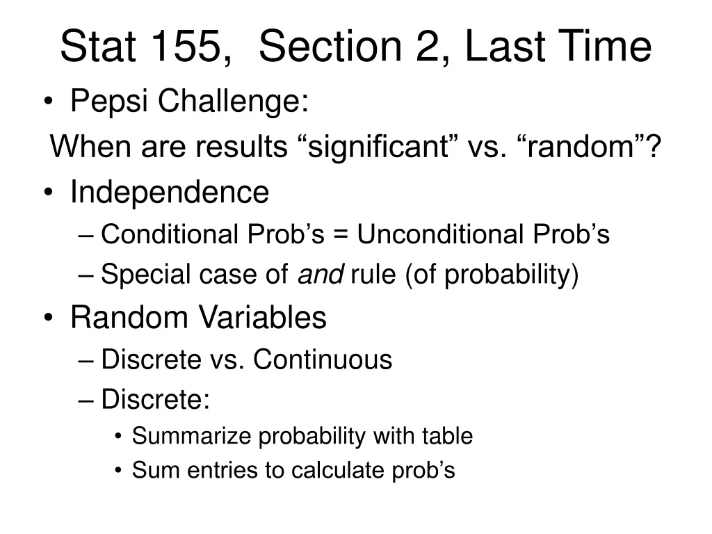
1. Stat 155, Section 2, Last Time • Pepsi Challenge: When are results “significant” vs. “random”? • Independence • Conditional Prob’s = Unconditional Prob’s • Special case of and rule (of probability) • Random Variables • Discrete vs. Continuous • Discrete: • Summarize probability with table • Sum entries to calculate prob’s

2. Reading In Textbook Approximate Reading for Today’s Material: Pages 277-286, 291-305 Approximate Reading for Next Class: Pages 291-305, 334-351

3. Midterm I Coming up: Tuesday, Feb. 27 Material: HW Assignments 1 – 6 Extra Office Hours: Mon. Feb. 26, 8:30 – 12:00, 2:00 – 3:30 (Instead of Review Session) Bring Along: 1 8.5” x 11” sheet of paper with formulas

4. Midterm I Suggestions for studying: • Exam based on HW, not text or class • Constructed by modifying HW problems • So rework HW problems Note: different from “looking over HW”

5. Midterm I Use Posted Old Exams: On Class Web Page • Least effective: read over solutions • Moderate: read test, think, then look • Best: Rework, then check

6. Midterm I Warning about Old Exams: • Have slightly less material • In particular probability not covered then • Because of different calendar (drop date used to be earlier) • Maybe something we haven’t covered • Clarify by email…

7. Midterm I Warning about Old Exams: • Famous last words…. “But I knew everything on the practice exam” • Practice exam only about “method” of questions • Not representative of material • Only a sample • As present exam will be

8. Random Variables Now consider continuous random variables Recall: for measurements (not counting) Model for continuous random variables: Calculate probabilities as areas, under “probability density curve”, f(x)

9. Continuous Random Variables Model probabilities for continuous random variables, as areas under “probability density curve”, f(x): = Area( ) a b (calculus notation)

10. Continuous Random Variables Note: Same idea as “idealized distributions” above Recall discussion from: Page 8, of Class Notes, Jan. 23

11. Continuous Random Variables e.g. Uniform Distribution Idea: choose random number from [0,1] Use constant density: f(x) = C Models “equally likely” To choose C, want: Area 1 = P{X in [0,1]} = C So want C = 1. 0 1

12. Uniform Random Variable HW: 4.54 (0.73, 0, 0.73, 0.2, 0.5) 4.56 (1, ½, 1/8)

13. Continuous Random Variables e.g. Normal Distribution Idea: Draw at random from a normal population f(x) is the normal curve (studied above) Review some earlier concepts:

14. Normal Curve Mathematics The “normal density curve” is: usual “function” of circle constant = 3.14… natural number = 2.7…

15. Normal Curve Mathematics Main Ideas: • Basic shape is: • “Shifted to mu”: • “Scaled by sigma”: • Make Total Area = 1: divide by • as , but never

16. Computation of Normal Areas EXCEL Computation: works in terms of “lower areas” E.g. for Area < 1.3

17. Computation of Normal Probs EXCEL Computation: probs given by “lower areas” E.g. for X ~ N(1,0.5) P{X < 1.3} = 0.73

18. Normal Random Variables As above, compute probabilities as areas, In EXCEL, use NORMDIST & NORMINV E.g. above: X ~ N(1,0.5) P{X < 1.3} =NORMDIST(1.3,1,0.5,TRUE) = 0.73 (as in pic above)

19. Normal Random Variables HW: 4.57, 4.58 (0.965, ~0)

20. And now for something completely different Recall Distribution of majors of students in this course:

21. And now for something completely different A photographer for a national magazine was assigned to get photos of a great forest fire. Smoke at the scene was too thick to get any good shots, so he frantically called his home office to hire a plane. "It will be waiting for you at the airport!" he was assured by his editor.

22. And now for something completely different As soon as he got to the small, rural airport, sure enough, a plane was warming up near the runway. He jumped in with his equipment and yelled, "Let's go! Let's go!" The pilot swung the plane into the wind and soon they were in the air.

23. And now for something completely different "Fly over the north side of the fire," said the photographer, "and make three or four low level passes.“ "Why?" asked the pilot. "Because I'm going to take pictures! I'm a photographer, and photographers take pictures!" said the photographer with great exasperation.

24. And now for something completely different After a long pause the pilot said, "You mean you're not the instructor?“ …

25. Means and Variances (of random variables) Text, Sec. 4.4 Idea: Above population summaries, extended from populations to probability distributions Connection: frequentist view Make repeated draws, from the distribution

26. Discrete Prob. Distributions Recall table summary of distribution: Taken on by random variable X, Probabilities: P{X = xi} = pi (note: big difference between X and x!)

27. Discrete Prob. Distributions Table summary of distribution: Recall power of this: Can compute any prob., by summing pi

28. Mean of Discrete Distributions Frequentist approach to mean:

29. Mean of Discrete Distributions Frequentist approach to mean: a weighted average of values where weights are probabilities

30. Mean of Discrete Distributions E.g. Above Die Rolling Game: Mean of distribution = = (1/3)(9) + (1/6)(0) +(1/2)(-4) = 3 - 2 = 1 Interpretation: on average (over large number of plays) winnings per play = $1 Conclusion: should be very happy to play

31. Mean of Discrete Distributions Terminology: mean is also called: “Expected Value” E.g. in above game “expect” $1 (per play) (caution: on average over many plays)

32. Expected Value HW: 4.59, 4.61

33. Expected Value An application of Expected Value: Assess “fairness” of games (e.g. gambling) Major Caution: Expected Value is not what is expected on one play, but instead is average over many plays. Cannot say what happens in one or a few plays, only in long run average

34. Expected Value E.g. Suppose have $5000, and need $10,000 (e.g. you owe mafia $5000, clean out safe at work. If you give to mafia, you go to jail, so decide to try to raise additional $5000 by gambling) And can make even bets, where P{win} = 0.48 (can really do this, e.g. bets on Red in roulette at a casino)

35. Expected Value E.g. Suppose have $5000, and need $10,000 and can make even bets, w/ P{win} = 0.48 Pressing Practical Problem: • Should you make one large bet? • Or many small bets? • Or something in between?

36. Expected Value E.g. Suppose have $5000, and need $10,000 and can make even bets, w/ P{win} = 0.48 Expected Value analysis: E(Winnings) = P{lose} x $0 + P{win} x $2 = 0.52 x $0 + 0.48 x $2 = = $0.96 Thus expect to lose $0.04 for every dollar bet

37. Expected Value E.g. Suppose have $5000, and need $10,000 and can make even bets, w/ P{win} = 0.48 Expect to lose $0.04 for every dollar bet • This is why gambling is very profitable (for the casinos, been to Las Vegas?) • They play many times • So expected value works for them • And after many bets, you will surely lose • So should make fewer, not more bets?

38. Expected Value E.g. Suppose have $5000, and need $10,000 and can make even bets, w/ P{win} = 0.48 Another view: StrategyP{get $10,000} one $5000 bet 0.48 ~ 1/2 two $2500 bets ~ (0.48)2 ~ 1/4 four $1250 bets ~ (0.48)2 ~ 1/16 “many” “no chance”

39. Expected Value E.g. Suppose have $5000, and need $10,000 and can make even bets, w/ P{win} = 0.48 Surprising (?) answer: • Best to make one big bet • Not much fun… • But best chance at winning Casino Folklore: • This really happens • Folks walk in, place one huge bet….

40. Expected Value Warning about Expected Value: Excellent for some things, but not all decisions e.g. if will play many times e.g. if only play once (so don’t have long run)

41. Expected Value Real life decisions against Expected Value: • State Lotteries • State sells tickets • Keeps about half of $$$ • Gives rest to ~ one (randomly chosen) player • So Expected Value is clearly negative • Why do people play? Totally irrational? • Players buy faint hope of humongous gain • Could be worth joy of thinking about it

42. Expected Value Real life decisions against Expected Value: • State Lotteries • Support ours in North Carolina? Interesting (and deep) philosophical balances: • Only totally voluntary tax • Yet tax burden borne mostly by poor • Is that fair? • Otherwise lose revenue to other states…

43. Expected Value Real life decisions against Expected Value: 2. Casino Gambling • Always lose in long run (expected value…) • Yet people do it. Are they nuts? • Depends on how many times they play • If really enjoy being ahead sometimes • Then could be worth price paid for the thrill • Serious societal challenge: (some are totally consumed by thrill)

44. Expected Value Real life decisions against Expected Value: 3. Insurance • Everyone pays about 2 x Expected Loss • Insurance Company keeps the rest! • So very profitable. • But e.g. car insurance is required by law! • Sensible, since if lose, can lose very big • Yet purchase is totally against Expected Value • OK, since you only play once (not many times) • Insurance Co’s play many times (Expected Value works for them) • So they are an evening out mechanism

45. And now for something completely different A Fun Movie Clip: 405 Landing – Video File

46. Functions of Expected Value Important Properties of the Mean: • Linearity: Why? i. e. mean “preserves linear transformations”

47. Functions of Expected Value Important Properties of the Mean: ii. summability: Why is harder, so won’t do here i. e. can add means to get mean of sums i. e. mean “preserves sums”

48. Functions of Expected Value E. g. above game: If we “double the stakes”, then want: “mean of 2X” Recall $1 before i.e. have twice the expected value

49. Functions of Expected Value E. g. above game: If we “play twice”, then have Same as above? But isn’t playing twice different from doubling stake? Yes, but not in means

50. Functions of Expected Value HW: 4.73