Download
1 / 12
130 likes | 156 Views
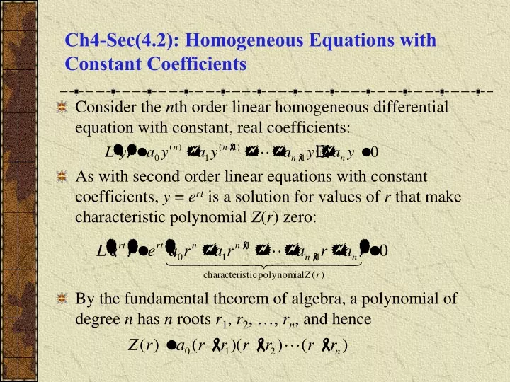
Ch4-Sec(4.2): Homogeneous Equations with Constant Coefficients. Consider the n th order linear homogeneous differential equation with constant, real coefficients:

E N D
Ch4-Sec(4.2): Homogeneous Equations with Constant Coefficients • Consider the nth order linear homogeneous differential equation with constant, real coefficients: • As with second order linear equations with constant coefficients, y = ert is a solution for values of r that make characteristic polynomial Z(r) zero: • By the fundamental theorem of algebra, a polynomial of degree n has n roots r1, r2, …, rn, and hence
Real and Unequal Roots • If roots of characteristic polynomial Z(r) are real and unequal, then there are n distinct solutions of the differential equation: • If these functions are linearly independent, then general solution of differential equation is • The Wronskian can be used to determine linear independence of solutions.
Example 1:Distinct Real Roots (1 of 3) • Consider the initial value problem • Assuming exponential soln leads to characteristic equation: • Thus the general solution is
Example 1:Solution (2 of 3) • The initial conditions yield • Solving, • Hence
Example 1: Graph of Solution (3 of 3) • The graph of the solution is given below. Note the effect of the largest root of the characteristic equation.
Complex Roots • If the characteristic polynomial Z(r) has complex roots, then they must occur in conjugate pairs, i. • Note that not all the roots need be complex. • Solutions corresponding to complex roots have the form • As in Chapter 3.4, we use the real-valued solutions
Example 2:Complex Roots (1 of 2) • Consider the initial value problem • Then • The roots are 1, -1, i, -i. Thus the general solution is • Using the initial conditions, we obtain • The graph of solution is given on right.
Example 2:Small Change in an Initial Condition (2 of 2) • Note that if one initial condition is slightly modified, then the solution can change significantly. For example, replace with then • The graph of this soln and original soln are given below.
Repeated Roots • Suppose a root rk of characteristic polynomial Z(r) is a repeated root with multiplicty s. Then linearly independent solutions corresponding to this repeated root have the form • If a complex root + i is repeated s times, then so is its conjugate - i. There are 2s corresponding linearly independent solns, derived from real and imaginary parts of or
Example 4: Repeated Roots • Consider the equation • Then • The roots are i, i, -i,-i. Thus the general solution is Sample Solution: y= (1 + t) Cos t + (1 + t) Sin t
Example 4: Complex Roots of -1 (1 of 2) For the general solution of , the characteristic equation is . To solve this equation, we need to use Euler’s equation to find the four 4th roots of -1: Letting m = 0, 1, 2, and 3, we get the roots:
Example 4: Complex Roots of -1 (2 of 2) • Given the four complex roots, extending the ideas from Chapter 4, we can form four linearly independent real solutions. • For the complex conjugate pair , we get the solutions • For the complex conjugate pair , we get the solutions • So the general solution can be written as