Download
1 / 22
220 likes | 232 Views
Learn how to calculate the bond amortization schedule and understand the adjustments made to the book value of a bond.

E N D
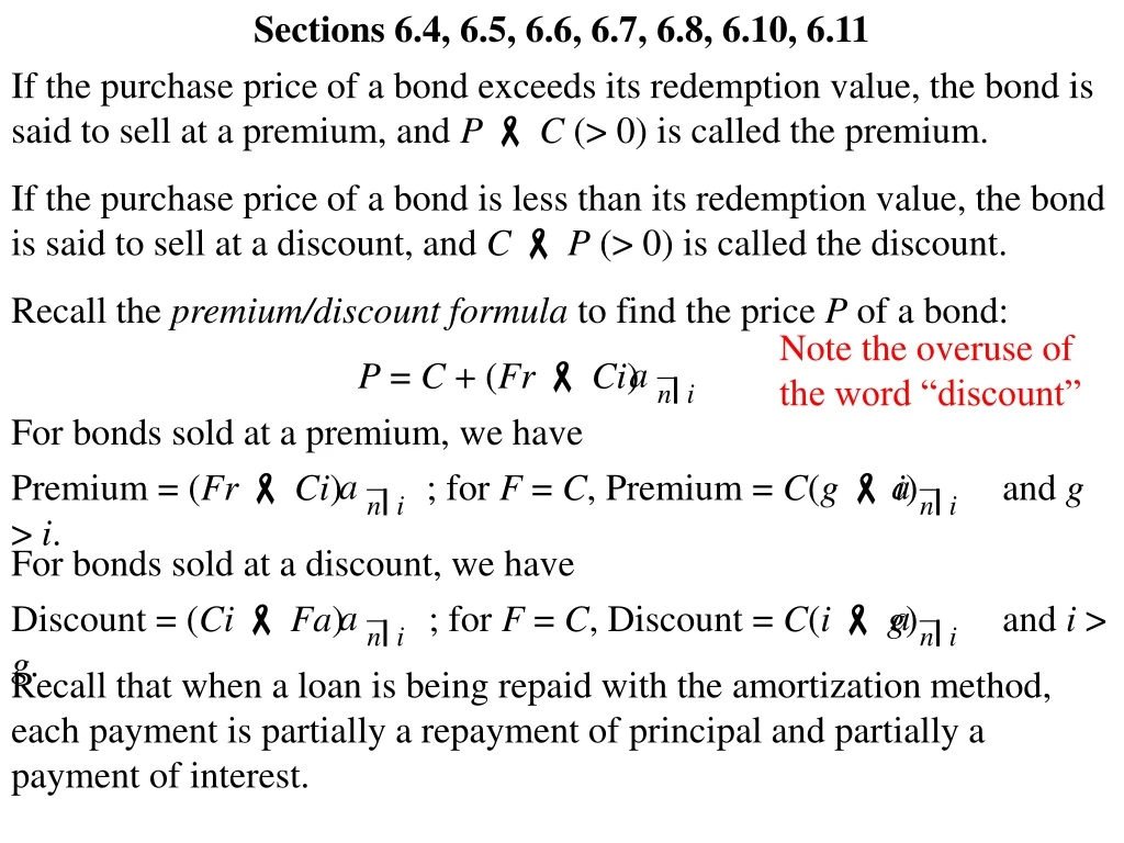
Sections 6.4, 6.5, 6.6, 6.7, 6.8, 6.10, 6.11 If the purchase price of a bond exceeds its redemption value, the bond is said to sell at a premium, and PC (> 0) is called the premium. If the purchase price of a bond is less than its redemption value, the bond is said to sell at a discount, and CP (> 0) is called the discount. Recall the premium/discount formula to find the price P of a bond: Note the overuse of the word “discount” P = C + (Fr Ci) a – n| i For bonds sold at a premium, we have Premium = (Fr Ci) ; for F = C, Premium = C(g i) and g > i. a – n| i a – n| i For bonds sold at a discount, we have Discount = (Ci Fa) ; for F = C, Discount = C(i g) and i > g. a – n| i a – n| i Recall that when a loan is being repaid with the amortization method, each payment is partially a repayment of principal and partially a payment of interest.
Suppose C = F (g = r) for a bond (i.e., the par value and redemption values are equal). The bond purchased for price P with yield rate i and redemption value C can be viewed as a loan/investment of P paid back with payments/returns equal to the periodic coupons and finally the redemption value at the end of the life of the bond. If P = C (g = i), then each coupon is interest on the loan/investment, and the redemption value is the principal. If PC (gi), then each coupon must be divided into interest earned and principal adjustment. A bond amortization schedule shows this division. When P > C, the principal adjustment will be downward, and when C > P, the principal adjustment will be upward. In the bond amortization schedule, the value of the bond is continually adjusted beginning at the price on the purchase date and ending at the redemption value on the redemption date; these adjusted values are called the book values of the bond. The book value at any time is not necessarily equal to the market value which can change as the prevailing interest rates change.
Let Bt be the book value after t periods. Then B0 = P and Bn = C. Suppose C = 1; then P = 1 + p where p = (g i) , and each coupon is g. a – n| i At the end of period 1, the interest earned on the balance at the beginning of the period is and the portion of the coupon that does not count as part of this interest, called the principal adjustment, is The book value at the end of the first period equals the book value at the beginning of the period minus the principal adjustment, which is iP = i[1 + (g i) ] , a – n| i (g i)vn . gi[1 + (g i) ] = gi (g i)(1 vn) = a – n| i B1 = B0 (g i)vn = [1 + (g i) ] (g i)vn = 1 + (g i) . a – n| i a ––– n 1| i Note that if the bond is sold at a premium, then the principal adjustment is lowering the book value, but if the bond is sold at a discount, then the principal adjustment is raising the book value.
By successively continuing this reasoning, an amortization table can be developed. Table 6.1 on page 208 of the textbook displays the format for such an amortization schedule. Observe each of the following from this table: 1. 2. 3. 4. The book values displayed on each line match the premium/discount formula to find the price at the original yield rate. The sum of the principal adjustment column is p = (g i) . a – n| i The sum of the interest earned column is the difference between the sum of the coupons and the sum of the principal adjustment column. The principal adjustment column is a geometric progression with common ratio 1 + i. The process of obtaining the book values in the last column is called writing up or writing down book values, depending on whether the book values are increasing or decreasing.
Bond X and Bond Y are each a two-year bond with a par value of $5000. Bond X has a coupon rate of 6% payable semiannually, and Bond Y has a coupon rate of 8% payable semiannually. Both bonds are to be brought to yield 7% convertible semiannually. It is easy to check (and this was done already in the handout for Sections 6.1, 6.2, 6.3) that the price for Bond X is $4908.17, and the price for Bond Y is $5091.83. (a) Complete the bond amortization schedule for Bond X below. Interest Earned Principal Adjustment Amount for Discount Book Value Period (Half-Year) Coupon 0 4908.17 1 150.00 171.79 21.79 4929.96 2 150.00 172.55 22.55 4952.51 3 150.00 173.34 23.34 4975.85 4 150.00 174.15 24.15 5000.00
(b) Complete the bond amortization schedule for Bond Y below. Interest Earned Principal Adjustment Amount for Premium Book Value Period (Half-Year) Coupon 0 5091.83 200.00 1 178.21 21.79 5070.04 177.45 22.55 5047.49 2 200.00 176.66 23.34 5024.15 200.00 3 175.85 24.15 5000.00 200.00 4 The process of obtaining the book values in the last column is called writing up or writing down book values, depending on whether the book values are increasing or decreasing. An approximate but simple method for writing up or writing down book values is the straight line method which sets the principal adjustment each period equal to (PC)/n and the interest earned each period equal to Fr (PC)/n .
For each of Bond X and Bond Y in the earlier exercise, list the book values that would result from the straight line method. For Bond X, the principal adjustment each period is (4908.17 5000)/4 = 22.9575 and the interest earned each period is 150 ( 22.9575) = 172.9575. The book values are 4908.17, 4931.13, 4954.085, 4977.04, 5000.00. For Bond Y, the principal adjustment each period is (5091.83 5000)/4 = 22.9575 and the interest earned each period is 150 22.9575 = 127.0425. The book values are 5091.83, 5068.87, 5045.915, 5022.96, 5000.00.
Investor/Purchaser/Lender receives periodic modified coupon payments on the “loan” from Issuer/Borrower P > C (g > i) implies a larger n is more favorable to the investor P < C (g < i) implies a larger n is more favorable to the issuer Investor/Purchaser/Lender “loans” amount P at time 0 Investor/Purchaser/Lender receives amount C at time n Issuer/Borrower receives amount P at time 0 Issuer/Borrower pays amount C at time n When a bond is sold at a premium, it can be said that the investor (purchaser or lender) experiences a loss equal to the premium at the redemption date; when a bond is sold at a discount, it can be said that the investor (purchaser or lender) experiences a profit equal to the discount at the redemption date. The profit or loss is reflected in the yield rate i. In the case where the bond is sold at a premium, suppose the investor is able to have the premium (loss) replaced by periodic deposits of the difference CgiP into a sinking fund earning interest rate j convertible at the same frequency as the yield rate i. Example 6.4 in the textbook gives the formula needed to appropriately adjust the price of the bond, and also provides a specific example.
Suppose we want to determine a price/book value for a bond between coupon payment dates t and t + 1. Let t + k be the time for which the price/book value is to be determined, i.e., 0 < k < 1. We define the following: Bt + k = market value of the bond, which is based on the present value of future coupons plus the present value of the redemption value minus a portion of the coupon payment at time t + 1 m Bt + k = flat price of the bond, which is the amount actually paid for the bond f time over which market value is based t t + k t + 1 n time over which portion of coupon payment at t + 1 is based to be subtracted from the market value.
Bt + k = market value of the bond, which is based on the present value of future coupons plus the present value of the redemption value minus a portion of the coupon payment at time t + 1 m Bt + k = flat price of the bond, which is the amount actually paid for the bond f Frk = accrued coupon, which is the portion of coupon payment at t + 1 to be subtracted from the market value, since the purchaser will receive the entire coupon payment at time t + 1 time over which market value is based t t + k t + 1 n time on which portion of coupon payment at t + 1 to be subtracted from the market value is based
We must have that Bt + k = Bt + k + Frk , or Bt + k = Bt + kFrk . There are three methods for computing these values: m m f f Flat Price Accrued Coupon Market Price Bt + k Frk Bt + k f m Bt(1 + i)k (1 + i)k 1 i Theoretical Method Bt(1 + i)k Fr (1 + i)k 1 i Fr Practical Method Bt(1 + ki) kFr Bt(1 + ki) kFr Semi-theoretical Method Bt(1 + i)k kFr Bt(1 + i)k kFr
Another issue which can be considered is the amount of premium or discount between coupon dates. This is easily calculated from Bt + k Cif g > i or from C Bt + k if i > g. m m From the amortization schedule of Bond X constructed earlier, use all three methods to find the flat price, accrued coupon, and market price for the bond four months after purchase. First, we calculate the following: Bt(1 + i)k = Bt(1 + ki) = Fr = kFr = B0(1 + 0.035)2/3 = (4908.17)(1.035)2/3 = $5021.86 (4908.17)(1 + (2/3)0.035) = B0(1 + (2/3)0.035) = $5022.52 (1.035)2/3 1 0.035 150 = $99.43 (1 + i)k 1 i (2/3)(150) = $100.00
First, we calculate the following: Bt(1 + i)k = Bt(1 + ki) = Fr = kFr = B0(1 + 0.035)2/3 = (4908.17)(1.035)2/3 = $5021.86 $5022.52 B0(1 + (2/3)0.035) = (1.035)2/3 1 0.035 150 = $99.43 (1 + i)k 1 i (2/3)(150) = $100.00 Flat Price Accrued Coupon Market Price B0 + 2/3 Fr2/3 B0 + 2/3 f m Theoretical Method $99.43 $5021.86 $4922.43 Practical Method $100.00 $5022.52 $4922.52 Semi-theoretical Method $100.00 $5021.86 $4921.86
From the amortization schedule of Bond Y constructed earlier, use all three methods to find the flat price, accrued coupon, and market price for the bond 13 months after purchase. First, we calculate the following: Bt(1 + i)k = Bt(1 + ki) = Fr = kFr = B2(1 + 0.035)1/6 = (5047.49)(1.035)1/6 = $5076.51 $5076.93 B2(1 + (1/6)0.035) = (5047.49)(1 + (1/6)0.035) = (1.035)1/6 1 0.035 200 = $32.86 (1 + i)k 1 i (1/6)(200) = $33.33
First, we calculate the following: Bt(1 + i)k = Bt(1 + ki) = Fr = kFr = B2(1 + 0.035)1/6 = (5047.49)(1.035)1/6 = $5076.51 $5076.93 B2(1 + (1/6)0.035) = (5047.49)(1 + (1/6)0.035) = (1.035)1/6 1 0.035 200 = $32.86 (1 + i)k 1 i (1/6)(200) = $33.33 Flat Price Accrued Coupon Market Price B2 + 1/6 Fr1/6 B2 + 1/6 f m Theoretical Method $32.86 $5076.51 $5043.65 Practical Method $33.33 $5076.93 $5043.60 Semi-theoretical Method $33.33 $5076.51 $5043.18
In practice, instead of using number of months, the exact number of days most likely would be used with the either the actual/actual method or the actual/360 method. Look at Example 6.6. The calculations in #1 and #2 are straightforward. Note how the calculations in #4 can be done with a TI calculator as follows: Press the APPS button, and selecting the Finance option. Select the TMV Solver option. Set N = 20, PV = 90, PMT = 4, FV = 100 Press the ALPHA button followed by the SOLVE button. These results should match the results in the example.
A callablebond is a bond for which the issuer (borrower) has an option to redeem prior to the normal maturity date. To calculate the price, assume that the issuer (borrower) will exercise the most advantageous option, which is least advantageous to the lender (investor): if the yield rate is less than the modified coupon rate (i.e., the bond sells at a premium), assume that the redemption date will be the earliest possible date, since the issuer (borrower) will prefer the lender (investor) experience the “loss of principle” as soon as possible; if the yield rate is greater than the modified coupon rate (i.e., the bond sells at a discount), assume that the redemption date will be the latest possible date, since the issuer (borrower) will prefer the lender (investor) experience the “gain of principle” as late as possible.
A putable (put) bond is a bond for which the owner (lender) has an option to redeem prior to the normal maturity date. To calculate a price, reverse the rules for callable bonds. For a given value if i, is an increasing function of n. Consequently, a callable bond will typically sell at a lower price (a higher yield rate) than an otherwise identical non-callable bond, and a putable bond will typically sell at a higher price (a lower yield rate) than an otherwise identical non-putable bond. a – n| i Look at Examples 6.8 and 6.9.
Serial bonds are a series of bonds with staggered redemption dates instead of a common maturity date. If the bonds are redeemable at m different dates, then the price, redemption value, and present value of the redemption value all corresponding to time t can be denoted respectively by Pt , Ct , and Kt for t = 1, 2, …, m. The valuation of the serial bonds is most efficiently done using Makeham’s formula on each bond in the series as follows: P1 + P2 + … + Pm = ggg K1 + (C1 K1) + K2 + (C2 K2) + … + Km + (Cm Km) = iii g K / + (C / K /) where i C / = C1 + C2 + … + Cm and K / = K1 + K2 + … + Km Look at Example 6.10.
Preferred stock and perpetual bonds are each types of fixed income securities without fixed redemption dates. The price must be equal to the present value of future dividends or coupons forever, i.e. the dividends/coupon form a perpetuity. The price is Fr P = . i Common stock is not a fixed income security, which implies dividends are not known in advance, and these dividends can fluctuate widely. The dividend discount model is based on obtaining a theoretical price by using projected dividends to calculate the present value of projected dividends. For instance, if a corporation is planning to pay a dividend of D at time 1, and it is projected that future periodic dividends will be paid indefinitely and will change geometrically with common ratio 1 + k where 1 < k < i(i.e., dividends increase at rate k if k > 0 and decrease at rate |k| if k < 0), then the theoretical price of the stock (from Chapter 4) is D . i k P = vD + v2(1 + k)D + v3(1 + k)2D + v4(1 + k)3D + … =
If a corporation is planning to pay a dividend of D at time 1, and it is projected that future periodic dividends will be paid up to and including at time n and will change geometrically with common ratio 1 + k where 1 < k < i, then the theoretical price of the stock (from Chapter 4) is P = vD + v2(1 + k)D + v3(1 + k)2D + v4(1 + k)3D + … + vn(1 + k)n1D = n 1 + k 1 1 + i D . i k Dividends on stocks in the United States are usually paid quarterly. Look at Example 6.14. Look at Example 6.15, and note the ambiguity in the description of the payments. The solution is based on the following payments: …
payments 2 2(1.05) 2(1.052) 2(1.053) 2(1.054) 2(1.055) 2(1.055)(1.025) 6 0 7 1 2 3 4 5 time payments 2(1.055)(1.0253) 2(1.055)(1.0255) 2(1.055)(1.0255) … 2(1.055)(1.0255) 2(1.055)(1.0255) 2(1.055)(1.0252) 2(1.055)(1.0254) 13 14 8 9 10 11 12 15 time Look at Example 6.16. Section 6.11 briefly describes the different approaches to valuation of securities on which universal agreement does not exist.