Download
1 / 1
10 likes | 106 Views
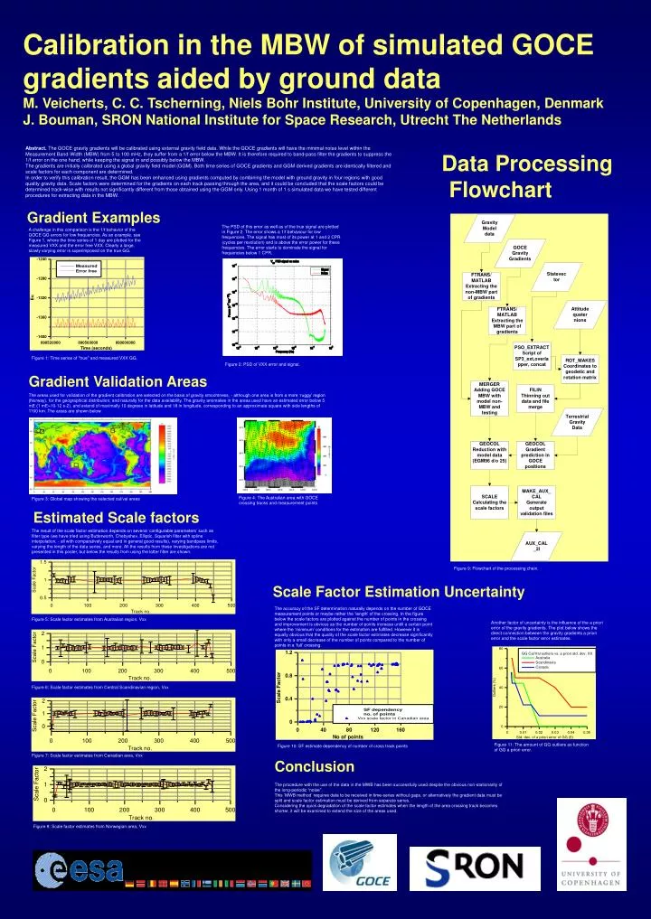
Calibration in the MBW of simulated GOCE gradients aided by ground data M. Veicherts, C. C. Tscherning, Niels Bohr Institute, University of Copenhagen, Denmark J. Bouman , SRON National Institute for Space Research, Utrecht The Netherlands.

E N D
Calibration in the MBW of simulated GOCE gradients aided by ground dataM. Veicherts, C. C. Tscherning, Niels Bohr Institute, University of Copenhagen, DenmarkJ. Bouman, SRON National Institute for Space Research, Utrecht The Netherlands Abstract. The GOCE gravity gradients will be calibrated using external gravity field data. While the GOCE gradients will have the minimal noise level within the Measurement Band-Width (MBW) from 5 to 100 mHz, they suffer from a 1/f error below the MBW. It is therefore required to band-pass filter the gradients to suppress the 1/f error on the one hand, while keeping the signal in and possibly below the MBW. The gradients are initially calibrated using a global gravity field model (GGM). Both time series of GOCE gradients and GGM derived gradients are identically filtered and scale factors for each component are determined. In order to verify this calibration result, the GGM has been enhanced using gradients computed by combining the model with ground gravity in four regions with good quality gravity data. Scale factors were determined for the gradients on each track passing through the area, and it could be concluded that the scale factors could be determined track-wise with results not significantly different from those obtained using the GGM only. Using 1 month of 1 s simulated data we have tested different procedures for extracting data in the MBW. Data Processing Flowchart Gradient Examples The PSD of this error as well as of the true signal are plotted in Figure 2. The error shows a 1/f behaviour for low frequencies. The signal has most of its power at 1 and 2 CPR (cycles per revolution) and is above the error power for these frequencies. The error starts to dominate the signal for frequencies below 1 CPR. A challenge in this comparison is the 1/f behavior of the GOCE GG errors for low frequencies. As an example, see Figure 1, where the time series of 1 day are plotted for the measured VXX and the error free VXX. Clearly a large, slowly varying error is superimposed on the true GG. Figure 1: Time series of "true" and measured VXX GG. Figure 2: PSD of VXX error and signal. Gradient Validation Areas The areas used for validation of the gradient calibration are selected on the basis of gravity smoohtness, - although one area is from a more ‘ruggy’ region (Norway), for the geographical distribution, and naturally for the data availability. The gravity anomalies in the areas used have an estimated error below 5 mE (1 mE=10-12 s-2), and extend of maximally 10 degrees in latitude and 18 in longitude, corresponding to an approximate square with side lengths of 1100 km. The areas are shown below. Figure 4: The Australian area with GOCE crossing tracks and measurement points Figure 3: Global map showing the selected cal/val areas Estimated Scale factors The result of the scale factor estimation depends on several ‘configurable parameters’ such as filter type (we have tried using Butterworth, Chebyshev, Elliptic, Squarish filter with spline interpolation, - all with comparatively equal and in general good results), varying bandpass limits, varying the length of the data series, and more. All the results from these investigations are not presented in this poster, but below the results from using the latter filter are shown. Figure 9: Flowchart of the processing chain. Scale Factor Estimation Uncertainty The accuracy of the SF determination naturally depends on the number of GOCE measurement points or maybe rather the ‘length’ of the crossing. In the figure below the scale factors are plotted against the number of points in the crossing and improvement is obvious as the number of points increase untill a certain point where the ‘minimum’ conditions for the estimation are fulfilled. However it is equally obvious that the quality of the scale factor estimates decrease significantly with only a small decrease of the number of points compared to the number of points in a ‘full’ crossing. Figure 5: Scale factor estimates from Australian region, Vxx Another factor of uncertainty is the influence of the a priori error of the gravity gradients. The plot below shows the direct connection between the gravity gradients a priori error and the scale factor error estimates. Figure 6: Scale factor estimates from Central Scandinavian region, Vxx Figure 11: The amount of GG outliers as function of GG a priori error. Figure 10: SF estimate dependency of number of cross track points Figure 7: Scale factor estimates from Canadian area, Vxx Conclusion The procedure with the use of the data in the MWB has been successfully used despite the obvious non-stationarity of the long-periodic “noise”. This ‘MWB method’ requires data to be received in time-series without gaps, or alternatively the gradient data must be split and scale factor estimation must be derived from separate series. Considering the quick degradation of the scale factor estimates when the length of the area crossing track becomes shorter, it will be examined to extend the size of the areas used. Figure 8: Scale factor estimates from Norwegian area, Vxx