Download

1 / 24
240 likes | 381 Views
1.3 EQUATION AND GRAPHS OF POLYNOMIAL FUNCTIONS. OBJECTIVES:. ZEROS (roots) of polynomial functions. ORDER E.g ) f(x) = (x+2) (x-1) 2 If (x-a n ), then the zeros of orders, is 2 at x= -1 and a double root. Value of x such that f(x) = 0 y-intercept = x = 0 x-intercept = y = 0.

E N D
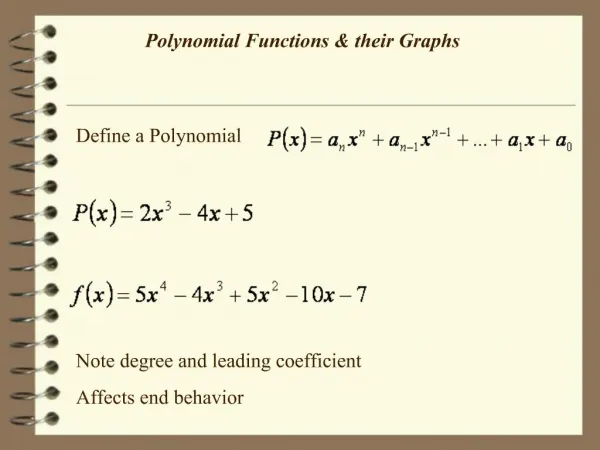
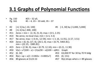
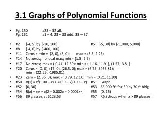
1.3 EQUATION AND GRAPHS OF POLYNOMIAL FUNCTIONS
OBJECTIVES: • ZEROS (roots) of polynomial functions. • ORDER • E.g) f(x) = (x+2) (x-1)2 • If (x-an), then the zeros of orders, is 2 at x= -1 and a double root. • Value of x such that f(x) = 0 • y-intercept = x = 0 • x-intercept = y = 0 Zeros(roots) Order X-intercept
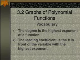
Examples: f(x) = -4x7 + 5x4 – 2x + 10 Leading Term Leading Coefficient Degree Term • Leading term : The term that the variable has • it’s highest opponent. In this case, the leading • term is -4x^7. • Leading Coefficient : The coefficient on the leading term. So, it would be -4. • Degree Term : The variable, which would be 7.
Example : (x-1) (x+1) GRAPHING A POLYNOMIAL FUNCTIONS Degree Sign Of leading Coefficient Y-intercept X-intercept Leading Point (n-1)
EVEN AND ODD FUNCTIONS • Even Function • Odd Function EVEN FUNCTION is when f(x) = f(-x), for all x. Symmetry on the y-axis Called even because… ODD FUNCTION is when -f(x) = f(-x), for all x. Origin Symmetry. Called odd because…
TRANSFORMMMEE!!!! All In One ... ! You can do all transformation in one go using this: a is vertical stretch/compression |a| > 1 = stretches |a| < 1= compresses a < 0= flips the graph upside down b= is horizontal stretch/compression |b| > 1 = compresses |b| < 1 =stretches b < 0 =flips the graph left-right c is= horizontal shift c < 0= shifts to the right c > 0= shifts to the left d =is vertical shift d > 0 =shifts upward d < 0 =shifts downward
Chapter 1 Polynomial Functions
1.1 Power Functions a = Coefficient (Real numbers) x = Variable n = Degree (must always be a whole number) All polynomial functions can be written in the form of:
Key Features of Graphs y = xn , n is even y = xn, n is odd
1.2 Characteristics of Polynomial Functions Finite Differences Method 2: Graphing Calculator Method 1: Pencil & Paper
Value of the Leading Coefficient FD = an! E.g. : 2 = a(1!) a = 2
Key Features of Graphs of Polynomial Functions with Odd Degree
Key Features of Graphs of Polynomial Functions with Even Degree
What is Rate of Change ??? Rate of change is a measure of the change in one quantity (the dependent variable) with respect to change in another quantity ( the independent variable)
Rate of Change • Average Rate of Change • A change that takes place over an interval. • Instantaneous Rate of Change • A change that takes place in an instant.
1.5 Slopes of Secant and Average Rate of Change Represents the rate of change over a specific interval . Corresponds to the slope of a secant between 2 points . Average Rate of Change formula: = y = y2-y1 x x2-x1 the slope between 2 points can be calculated by : A table of values An equation .
Examples Example 1 : A new antibacterial spray is tested on a bacterial culture. The table shows the population, P, of the bacterial culture t, minutes after the spray is applied. Determine the average rate of change. From the table with the points (0,800) and (7,37): Average rate of change =P = 37-800 = -109 t 7-0 During the entire 7 minutes , the number of bacteria decreases on average by 109 bacteria per minute.
A football is kicked into the air such that its height ,h, in metres, after t seconds can be modelled by the function h(t) =-4.9 t2 + 14t +1. Determine the average rate of change of the height for the time interval : [0 , 0.5 ] • Example 2 : Solution : Substitute t=0 , h(0)= -4.9(0)2 + 14 (0) + 1=1 Substitute t= 0.5, h(0.5)=-4.9(0.5)2 + 14(0.5) +1 =6.775 Average rate of change = h = 6.775-1 = 11.55 t 0.5-0 The average rate of change of the height of the football from 0s to 0.5s is 11.55m/s.
1.6 Instantaneous Rate of Change • An instantaneous rate of change corresponds to the slope of a tangent to a point on a curve . • An approximate value can be determined by : 1. A graph • Draw a tangent line on the graph and estimating the slope of the tangent of the graph. 2. A table of values • Estimating the point and a nearby point in the table 3. An equation • Estimating the slope using a very short interval between the tangent point and a second point found using the equation
Example : Graph method The function shows a ball thrown into the air according to the equation f(x) = -5x2 + 10x ; where x is time (s) and f is height (m) . Find the instantaneous rate of change of the ball at 1.5 seconds in different ways .