Download
1 / 51
510 likes | 718 Views
SLP Cyclone anti-cyclone asymmetry and time mean field. July 8, 2008. NCEP reanalysis 1948-2008, DJF No filtering. NH Time mean (raw) reflected about equator. Total wavenumber >=6. Normalized by STD^3. Skewness (contours) Time mean (colors. Example Fit. Histograms of extrema.

E N D
SLPCyclone anti-cyclone asymmetryand time mean field July 8, 2008
NCEP reanalysis 1948-2008, DJF No filtering
NH Time mean (raw) reflected about equator Total wavenumber >=6
Skewness (contours) Time mean (colors
Histograms of extrema • Locate local (time) extrema in daily time series at each gridpoint • Can use a threshold to define unique extrema (doesn’t change much of the results) • Compile the histograms of positive and negative extrema • Do these look the same as raw data histogram?
Tracking of SLP • All data is NCEP mean SLP from 1978-2008 DJFM, daily • Two pre-filtering routines are comparesd • Spatial filter that keeps total planetary wavenumber >= 6 (Hoskins); • A temporal, high pass filter (double pass, sixth order butterworth) with cutoff period of 20 days.
Define Regions over which the time mean, spatially filtered field is large
Can we explain the histogram differences by simple adding a time mean to the temporal data • Find the spatial average of the spatially filtered time mean SLP in each boxed domain • Add this constant to all the tracked data magnitudes • Compute the histograms alongside the spatially filtered tracked data
TRACKS AND COMPOSITES BY REGION • Take the 100 largest storms in each region (that way number of tracked features doesn’t get in the way) • Plot tracks, all is lagrangrian data defined by the filter used • Composite around the 100 features onto the RAW SLP Eulerian fields relative to storm center • In plots, the spatial mean of the composite field is subtracted for visual purposes.
Look in the middle of the Atlantic, where there is a node in the mean