Download
1 / 31
310 likes | 451 Views
BIO/CS 471 – Algorithms for bioinformatics. Graph Theoretic Concepts and Algorithms for Bioinformatics. a. b. c. a. b. c. What is a “graph”. Formally: A finite graph G ( V , E ) is a pair ( V , E ), where V is a finite set and E is a binary relation on V .

E N D
BIO/CS 471 – Algorithms for bioinformatics Graph Theoretic Concepts and Algorithmsfor Bioinformatics
a b c a b c What is a “graph” • Formally: A finite graph G(V, E) is a pair (V, E), where V is a finite set and E is a binary relation on V. • Recall: A relationR between two sets X and Y is a subset of X x Y. • For each selection of two distinct V’s, that pair of V’s is either in set E or not in set E. • The elements of the set V are called vertices (or nodes) and those of set E are called edges. • Undirected graph: The edges are unordered pairs of V (i.e. the binary relation is symmetric). • Ex: undirected G(V,E); V = {a,b,c}, E = {{a,b}, {b,c}} • Directed graph (digraph):The edges are ordered pairs of V (i.e. the binary relation is not necessarily symmetric). • Ex: digraph G(V,E); V = {a,b,c}, E = {(a,b), (b,c)}
Why graphs? • Many problems can be stated in terms of a graph • The properties of graphs are well-studied • Many algorithms exists to solve problems posed as graphs • Many problems are already known to be intractable • By reducing an instance of a problem to a standard graph problem, we may be able to use well-known graph algorithms to provide an optimal solution • Graphs are excellent structures for storing, searching, and retrieving large amounts of data • Graph theoretic techniques play an important role in increasing the storage/search efficiency of computational techniques. • Graphs are covered in section 2.2 of Setubal & Meidanis
R Y L I Graphs in bioinformatics • Sequences • DNA, proteins, etc. Chemical compounds Metabolic pathways
Graphs in bioinformatics Phylogenetic trees
Basic definitions • incidence: an edge (directed or undirected) is incident to a vertex that is one of its end points. • degree of a vertex: number of edges incident to it • Nodes of a digraph can also be said to have an indegree and an outdegree • adjacency: two vertices connected by an edge are adjacent Undirected graph Directed graph loop loop G=(V,E) isolated vertex adjacent multiple edges
x y “Travel” in graphs a path: no vertex can be repeated example path: a-b-c-d-e trail: no edge can be repeated example trail: a-b-c-d-e-b-d walk: no restriction example walk: a-b-d-a-b-c closed: if starting vertex is also ending vertex length: number of edges in the path, trail, or walk circuit: a closed trail (ex: a-b-c-d-b-e-d-a) cycle: closed path (ex: a-b-c-d-a) e b d c
Simple graph a e b d a c e b K5 d c Types of graphs • simple graph: an undirected graph with no loops or multiple edges between the same two vertices • multi-graph: any graph that is not simple • connected graph: all vertex pairs are joined by a path • disconnected graph: at least one vertex pairs is not joined by a path • complete graph: all vertex pairs are adjacent • Kn: the completely connected graph with n vertices Disconnected graph with two components
a b 10 5 c d 8 -3 2 e f 6 Types of graphs • acyclic graph (forest): a graph with no cycles • tree: a connected, acyclic graph • rooted tree: a tree with a “root” or “distinguished” vertex • leaves: the terminal nodes of a rooted tree • directed acyclic graph (DAG): a digraph with no cycles • weighted graph: any graph with weights associated with the edges (edge-weighted) and/or the vertices (vertex-weighted)
Digraph definitions • for digraphs only… • Every edge has a head(starting point) and a tail (ending point) • Walks, trails, and paths can only use edges in the appropriate direction • In a DAG, every path connects an predecessor/ancestor (the vertex at the head of the path) to its successor/descendents (nodes at the tail of any path). • parent: direct ancestor (one hop) • child: direct descendent (one hop) • A descendent vertex is reachablefrom any of its ancestors vertices Directed graph a b c d x y w v u z
6 c b 2 8 10 4 a d Computer representation • undirected graphs: usually represented as digraphs with two directed edges per “actual” undirected edge. • adjacency matrix: a |V| x |V| array where each cell i,j contains the weight of the edge between vi and vj (or 0 for no edge) • adjacency list: a |V| array where each cell i contains a list of all vertices adjacent to vi • incidence matrix: a |V| by |E| array where each cell i,j contains a weight (or a defined constant HEAD for unweighted graphs) if the vertex i is the head of edge j or a constant TAIL if vertex I is the tail of edge j adjacency list incidence matrix adjacency matrix
Class Node: label = NIL; parents = []; # list of nodes coming into this node children = []; # list of nodes coming out of this node childEdgeWeights = []; # ordered list of edged weights Computer representation • Linked list of nodes: Node is a defined data object with labels which include a list of pointers to its children and/or parents • Graph = [] # list of nodes
a e b e b d c d c Subgraphs • G’(V’,E’) is a subgraph of G(V,E) if V’ V and E’ E. • induced subgraph: a subgraph that contains all possible edges in E that have end points of the vertices of the selected V’ a d c Induced subgraph of G with V’ = {b,c,d,e} G(V,E) G’({a,c,d},{{c,d}})
a G G e b a e b d c d c Complement of a graph • The complement of a graph G (V,E) is a graph with the same vertex set, but with vertices adjacent only if they were not adjacent in G(V,E)
6 c b 2 8 10 4 a d Famous problems: Shortest path • Consider a weighted connected directed graph with a distinguished vertex source: a distinguished vertex with zero in-degree • What is the path of total minimum weight from the source to any other vertex? • Greedy strategy works for simple problems (no cycles, no negative weights) • Longest path is a similar problem (complement weights) • We will see this again soon for fragment assembly! Dijkstra (G (V,E,W)) { s0 = 0; for (I = 1 to n) si = w0,i; repeat { Select an unmarked vertex vq such that sq is minimal; Mark vq; foreach (unmarked vertex vi) si = min {si, (sq + wq,i)}; } until (all vertices are marked); }
1 a 2 3 e b 4 5 d c Famous problems: Isomorphism • Two graphs are isomorphic if a 1-to-1 correspondence between their vertex sets exists that preserve adjacencies • Determining to two graphs are isomorphic is NP-complete
1 2 4 3 Famous problems: Maximal clique • clique: a complete subgraph • maximal clique: a clique not contained in any other clique; the largest complete subgraph in the graph • Vertex cover: a subset of vertices such that each edge in E has at least one end-point in the subset • clique cover: vertex set divided into non-disjoint subsets, each of which induces a clique • clique partition: a disjoint clique cover Maximal cliques: {1,2,3},{1,3,4} Vertex cover: {1,3} Clique cover: { {1,2,3}{1,3,4} } Clique partition: { {1,2,3}{4} }
1 2 4 3 Famous problems: Coloring • vertex coloring: labeling the vertices such that no edge in E has two end-points with the same label • chromatic number: the smallest number of labels for a coloring of a graph • What is the chromatic number of this graph? • Would you believe that this problem (in general) is intractable?
a 3 e 1 b 3 2 4 3 d 5 4 2 c c a b e d f h g i Famous problems: Hamilton & TSP • Hamiltonian path: a path through a graph which contains every vertex exactly once • Finding a Hamiltonian path is another NP-complete problem… • Traveling Salesmen Problem (TSP): find a Hamiltonian path of minimum cost
K4,4 Famous problems: Bipartite graphs • Bipartite: any graph whose vertices can be partitioned into two distinct sets so that every edge has one endpoint in each set. • How colorable is a bipartite graph? • Can you come up with an algorithm to determine if a graph is bipartite or not? • Is this problem tractable or intractable?
e b d f a h 1 2 c g 4 3 Famous problems: Minimal cut set • cut set: a subset of edges whose remove causes the number of graph components to increase • vertex separation set: a subset of vertices whose removal causes the number of graph components to increase • How would you determine the minimal cut set or vertex separation set? cut-sets: {(a,b),(a,c)}, {(b,d),(c,d)},{(d,f)},...
a b c d e f Famous problem: Conflict graphs • Conflict graph: a graph where each vertex represents a concept or resource and an edge between two vertices represents a conflict between these two concepts • When the vertices represents intervals on the real line (such as time) the conflict graph is sometimes called an interval graph • A coloring of an interval graph produces a schedule that shows how to best resolve the conflicts… a minimal coloring is the “best” schedule” • This concept is used to solve problems in the physical mapping of DNA Colors?
e b d f a 2 2 h 6 4 8 2 4 c g 4 1 2 Famous problems: Spanning tree • spanning tree: A subset of edges that are sufficient to keep a graph connected if all other edges are removed • minimum spanning tree: A spanning tree where the sum of the edge weights is minimum e b 2 2 6 d 8 f a 2 h 4 4 1 2 c g
area b area d area c a b d c Famous problems: Euler circuit • G is said to have a Euler circuit if there is a circuit in G that traverses every edge in the graph exactly once • The seven bridges of Konigsberg: Find a way to walk about the city so as to cross each bridge exactly once and then return to the starting point. This one is in P!
… … … … … … a a a a a a b b b b b b c c c c c c y y y y y y z z z z z z Famous problems: Dictionary • How can we organize a dictionary for fast lookup? 26-ary “trie” “CAB”
1 a 3 c b 2 6 4 5 7 f e d Graph traversal • There are many strategies for solving graph problems… for many problems, the efficiency and accuracy of the solution boil down to how you “search” the graph. • We will consider a “travel” problem for example: • Given the graph below, find a path from vertex a to vertex d. Shorter paths (in terms of edge weight sums) are desirable.
1 a 3 c b 2 6 4 5 7 f e d A greedy approach • greedy traversal: Starting with the “root” node, take the edge with smallest weight. Mark the edge so that you never attempt to use it again. If you get to the end, great! If you get to a dead end, back up one decision and try the next best edge. • Advantages: Fast! Drawbacks: Answer is usually non-optimal • For some problems, greedy approaches are optimal, for others the answer may usually be close to the best answers, for yet other problems, the greedy strategy is a poor choice. Start node: a End node: d Traversal order: a, c, f, e, b, d
1 a 3 c b 2 6 4 5 7 f e d Exhaustive search: Breadth-first • For the current node, do any necessary work • In this case, calculate the cost to get to the node by the current path; if the cost is better than any previous path, update the “best path” and “lowest cost”. • Place all adjacent unused edges in a queue (FIFO) • Take an edge from the queue, mark it as used, and follow it to the new current node Traversal order: a, b, c, d, e, f
1 a 3 c b 2 6 4 5 7 f e d Exhaustive search: Depth-first • For each current node • do any necessary work • Pick one unused edge out and follow it to a new current node • If no unused edges exist, unmark all of your edges an go back from whence you came! • DFS (G, v) • V.state = “visited” • Process vertex v • Foreach edge (v,w) { • if w.state = “unseen” { • DFS (G, w) • process edge (v,w) • } • } • } Traversal order: a, b, d, e, f, c
1 a 3 c b 2 6 4 5 7 f e d Branch and Bound • Begin a depth-first search (DFS) • Once you achieve a successful result, note the result as our initial “best result” • Continue the DFS; if you find a better result, update the “best result” • At each step of the DFS compare your current “cost” to the cost of the current “best result”; if we already exceed the cost of the best result, stop the downward search! Mark all edges as used, and head back up. Traversal order: Path Current Best A 0 - AE 2 - AEB 6 - AEBD 11 11 AEF 9 11 AEFC 15 11 AC 1 11 Path Current Best ACF 7 11 ACFE 15 11 < prune AB 3 11 ABD 8 8 ABE 7 8 ABEF 14 8
5 8 3 9 2 4 6 10 1 7 Binary search trees • Binary trees have at two children per node (the child may be null) • Binary search trees are organized so that each node has a label. • When searching or inserting a value, compare the target value to each node; one out-going edge corresponds to “less than” and one out-going edge corresponds to “greater than”. • On the average, you eliminate 50% of the search space per node… if the tree is balanced