Download
1 / 33
340 likes | 539 Views
Cognitive Engineering PSYC 530 Signal Detection. Raja Parasuraman. Overview. The Generalized Diagnostic Decision Making Problem Signal Detection Theory: Sensitivity and Criterion Derivation from first principles Equations d’, ß, and the ROC curve Examples.

E N D
CognitiveEngineeringPSYC 530Signal Detection Raja Parasuraman
Overview • The Generalized Diagnostic Decision Making Problem • Signal Detection Theory: Sensitivity and Criterion • Derivation from first principles • Equations • d’, ß, and the ROC curve • Examples
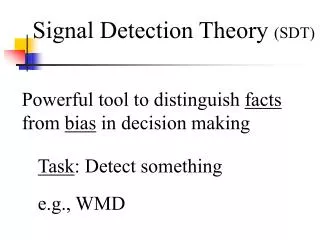
The Generalized Diagnostic Decision Making Problem • Determining whether (Yes) or not (No) a certain condition exists (or will occur) • Making this determination in the face of uncertain or incomplete evidence • While the real world often contains cases with multiple alternatives, the problem of distinguishing between two alternatives, or “States of the World” is sufficiently general for many applications.
Detecting Signals in Human-Machine Systems • Air traffic control: Are the 2 aircraft in “conflict” (within 5 miles or 1,000 ft. of each other) or not? • Industrial inspection and quality control: Does a manufactured product have a specified flaw or not? • Medical imaging: Does the MRI scan show a tumor or not? • Baggage screening: Is the object in the bag a weapon or not?
Evaluating Diagnostic Systems • Does an ATC decision aid improve the controller’s accuracy in detecting aircraft conflicts? • Does a particular training regimen improve quality control of a manufactured product? • Does color coding and contrast enhancement increase radiologist sensitivity to tumor detection? • Are baggage screeners with high spatial ability more accurate in weapon detection?
Diagnostic Accuracy and Systems Design I. “Fitting the Machine to the Human”: Display control, and interface design • Does an ATC decision aid improve the controller’s accuracy in detecting aircraft conflicts? • Does a particular training regimen improve quality control of a manufactured product? • Does color coding and contrast enhancement increase radiologist sensitivity to tumor detection? • Are baggage screeners with high spatial ability more accurate in weapon detection? II. “Fitting the Human to the Machine”: Selection and training
The Decision Matrix State of the World Signal Noise Yes Response No
Terms, Terms, Terms! State of the World Signal Noise P(H)=H/S Yes Positive P(FA)=FA/N Response P(M)=M/S= 1- P(H) No Negative P(CR)=CR/N= 1- P(FA) S N Only two cells are needed to characterize the decision matrix Typically, Hit Rate or P(H) and FA Rate or P(FA) are used
Detection Sensitivity System or Condition A System or Condition B S N S N Yes No 100 100 100 100 Which System, A or B, has higher detection sensitivity?
Options for Evaluating Sensitivity System or Condition A System or Condition B S N S N Yes No 100 100 100 100 Hit or True Positive Rate: 90% vs 60%: A > B False Alarm or False Positive Rate: 25% vs 5%: B > A OverallCorrect [90%+75%]/2 vs [60%+95%]/2=82.5% vs 77.5%: A>B All of the above are biased measures of sensitivity
Sensitivity and Criterion Both the hit rate (or hit probability) and the false alarm rate (or FA probability) need to be considered in order to compute sensitivity and criterion. Sensitivity (detectability, discriminability, “accuracy”) refers to the ability to distinguish signal from noise, independent of the tendency to emit a positive or negative response Criterion (response bias, response threshold) refers to the tendency to emit a positive response Hence in the previous example, the pair {.9,.25} has to be compared to the pair {.6,.05}. How? Signal detection theory.
Sensitivity and Criterion • The key to comparing pairs of numbers • (hit rate, false alarm rate) is to under- • stand that each reflects the joint • influence of two factors, sensitivity— • the basic ability to distinguish signal • from noise—and criterion—the • tendency to emit one response (e.g., Yes) • over the other. • Neither hit rate nor false alarm rate nor overall correct provide a true, unbiased measure of sensitivity. • Signal detection theory provides unbiased, • independent measures of sensitivity (d’) and criterion (ß). Yes No {.9,.25} vs {.6,.05} Which is better?
Understanding the Criterion: A Coin Tossing Game Toss a fair coin 200 times States of the world: 100 Heads, 100 Tails Task: Predict whether the coin will land “Heads” Liberal Criterion: Always Say “Heads”--“Cry Wolf” Strategy Conservative Criterion” Never Say “Heads”--“Cautious” Strategy Heads Tails Heads Tails Say “Heads” Say “Tails” 100 100 100 100 Outcome: 0% “FA” rate but at the cost of a 0% “Hit” rate Outcome: 100% “Hit” rate but at the cost of a 100% “FA” rate
Factors Influencing the Criterion Decision Criterion Continuum Extreme Liberal: 100% H, 100%FA Extreme Conservative: 0% H, 0% FA • The prior probability (or base rate) of a signal • Low prior probability: Conservative criterion (e.g., medical screening) • High prior probability: Liberal criterion (e..g, medical referral) • Equal prior probability of S and N (50-50): Neutral or unbiased criterion (e.g., coin-tossing game; experiment in perception or memory) • The costs and values attached to the four decision outcomes (H, FA, M, CR) • High value for H: Liberal • High cost for FA: Conservative • High cost for M: Liberal • High value for CR: Conservative X% H, y% FA
Factors Influencing Sensitivity • The signal to noise ratio • Basic sensory and cognitive ability • other factors
The ROC (Receiver Operating Characteristic) Perfect sensitivity Moderate sensitivity Extreme liberal 1.0 P(H) Coin tossing game: Zero sensitivity 0 Extreme conservative P(FA) 1.0
1.0 Varying Criterion, Fixed Sensitivity P(H) 0 1.0 Increasing Sensitivity P(H) 0 P(FA) 1.0 The ROC (Receiver Operating Characteristic) The ROC is the locus of H and FA probabilities as the decision criterion varies for a given, fixed level of sensitivity. P(FA) 1.0 Different levels of sensitivity are represented on different ROCs. The higher the sensitivity, the more to the left the ROC is bowed, reaching perfect sensitivity at a {P(H), P(FA} of {1,0}
Distinguishing Sensitivity between Conditions A and B Condition A: {.9, .25} If A lies on a higher ROC than B, sensitivity for A is higher than that for B (or vice versa) If A and B lie on the same ROC, then A and B have equal sensitivity and the differences in P(H) and P(FA) between conditions are solely due to criterion variation 1.0 P(H) 0 1.0 P(FA) Condition B: {.6, .05}
Signal Detection Theory “No” “Yes” Noise Distribution Signal Distribution Criterion Level Zc “Evidence” A Random Variable Z Decision Rule: If the evidence on any given trial exceeds the criterion level evidence Zc, then say “Yes”, otherwise say “No”
SDT is related to Basic Stats Stuff! (Ho, H1, Rejecting the Null Hypothesis, Type I and II Errors, etc.) P(H) = Probability of Yes given Signal = Area Under Signal Distribution to the Right of the Criterion “No” “Yes” Signal Distribution Noise Distribution P(FA) = Probability of Yes given Noise = Area Under Noise Distribution to the Right of the Criterion
Effects on P(H) and P(FA) of Varying the Criterion at Fixed Sensitivity Varying Criterion Yes”“ P(H) P(FA) Extreme Liberal P(H) = 1 P(FA) = 1 Extreme Conservative P(H) = 0 P(FA) = 0 1.0 Varying Criterion, Fixed Sensitivity P(H) 0
Varying Sensitivity Zero (coin-tossing game) Low Sensitivity = Distance between S and N distributions High Perfect In theory, infinite
Calculating Sensitivity and Criterion • Signal Detection Theory assumptions • Normal (Gaussian) distributions of evidence given signal (S) or noise (N) • Equal variance of signal and noise distributions • Sensitivity d’ is the distance between the means of the S and N distributions; can be estimated from the P(H) and P(FA) probabilities and their associated Z (normalized) values • The decision criterion ß is the ratio (at the criterion level) of the likelihood of a signal vs. that for noise; can be estimated from the Y values (heights) associated with P(H) and P(FA)
d’ N S Z(FA) -Z(H) Caculating Sensitivity Sensitivity: d’ = Z(FA) - Z(H) (For the convention that Z() is positive for p <.5 and negative for p>.5)
N S Y(H) Y(FA) Extreme Liberal ß = Extreme Conservative ß = 0 Unbiased or Neutral ß = 1 Criterion: ß = Y(H)/Y(FA) Caculating Criterion
Z = the normal deviate P = the area under the normal distribution corresponding to a given Z value Y = the ordinate (height) of the normal distribution for a given Z value Z can vary from + infinity (+∞) through 0 to - infinity (-∞), whereas P can vary from 0 to 1. Convention for conversions from P to Z and vice versa: If P isless than 0.5 Z is positive The Normal Curve If P isgreater than 0.5 Z is negative
Examples • P(H) = .9; P(FA) = .25 (Condition A) d’ = Z(FA) - Z(H) = Z(.25) - Z(.9) = 0.675 - (-Z(.1)) = 0.675 - (-.1.282) = 1.957 (Condition A) • P(H) = .6; P(FA) = .05 (Condition B) d’ = Z(FA) - Z(H) = Z(.05) - Z(.6) = 1.645 - (-Z(.4)) = 1.645 - (-.253) = 1.898 (Condition B) • Condition A is very slightly higher than Condition B (probably not significantly different in statistical test) • ß = Y(H)/Y(FA) = Y(.9)/Y(.25) • = Y(.1)/Y(.25) = .176/.318 = .553(Condition A; liberal) • ß = Y(H)/Y(FA) = Y(.6)/Y(.05) = Y(.4)/Y(.05) = .386/.103 = 3.748(Condition B; conservative)
Values of Sensitivity • d’ = 0 Chance level; Zero sensitivity • d’ = 1 Very Low; Very Difficult detection • d’ = 2 Low-Moderate; Difficult detection • d’ = 3 Moderate-High; Easier detection • d’ = 4 High; Easy detection • d’ = 5 Very High; Very easy detection • d’ > 6 Usually impossible to measure Why? For P(H) = .999 and P(FA) = .001 (1 miss and 1 FA in 1000 trials) d’ = 6.181
Values of Criterion • ß < 1 Liberal (In the extreme ß = 0) • ß = 1 Unbiased • ß > 1 Conservative (In the extreme ß = ) • Values from .1 to 50 are typically possible • Unbalanced scale (01 ); sometimes use Log ß • Log ß varies from - through 0 (unbiased) to +
Non-parametric Measure of Sensitivity 1.0 A=Area Under ROC P(H) 0 P(FA) 1.0 A varies from 0.5 (chance level) to 1.0 (perfect sensitivity)
A Recent Application of SDT: Homeland Security A Threat Display Concept for Radiation Detection in Homeland Security Cargo Screening Thomas F. Sanquist, Pamela Doctor Pacific Northwest National Laboratory Raja Parasuraman George Mason University
RPM = Radiation Portal Monitoring SDT Analysis of Detection and Classification