Download

1 / 36
360 likes | 364 Views
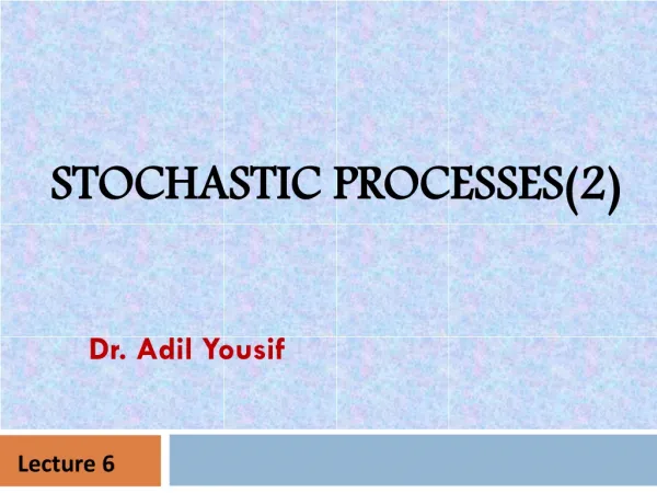
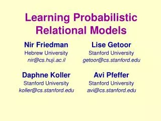
Learning Models of Relational Stochastic Processes. Sumit Sanghai. P2. P1. P3. V1. A1. A2. Motivation. Features of real-world domains Multiple classes, objects, relations. P2. ?. P1. P3. V1. A1. A2. ?. ?. Motivation. Features of real-world domains

E N D
Learning Models of Relational Stochastic Processes Sumit Sanghai
P2 P1 P3 V1 A1 A2 Motivation • Features of real-world domains • Multiple classes, objects, relations
P2 ? P1 P3 V1 A1 A2 ? ? Motivation • Features of real-world domains • Multiple classes, objects, relations • Uncertainty
Motivation • Features of real-world domains • Multiple classes, objects, relations • Uncertainty • Changes with time P5 P2 P6 P1 P3 V1 P4 A3 A1 A2
Relational Stochastic Processes • Features • Multiple classes, objects, relations • Uncertainty • Change over time • Examples: Social networks, molecular biology, user activity modeling, web, plan recognition, … • Growth inherent or due to explicit actions • Most large datasets are gathered over time • Explore dependencies over time • Predict future
Paint(A, blue) Manufacturing Process
Paint(A, blue) Bolt(B, C) Manufacturing Process
A.col A.col P t t + 1 red red 0.1 red blue 0.9 blue blue 0.95 blue red 0.05 Manufacturing Process Paint(A, blue) Bolt(B, C)
Why are they different? • Modeling object, relationships modification, creation and deletion • Modeling actions (preconditions/effects), activities, plans • Can’t just throw ``time’’ into the mix • Summarizing object information • Learning can be made easier by concentrating on temporal dependencies • Sophisticated inference techniques like particle filtering may be applicable
Outline • Background: Dynamic Bayes Nets • Dynamic Probabilistic Relational Models • Inference in DPRMs • Learning with Dynamic Markov Logic Nets • Future Work
X1t+1 X1t X2t X2t+1 Yt+1 Yt t t+1 Dynamic Bayesian Networks • DBNs model change in uncertain variables over time • Each time slice consists of state/observation variables • Bayesian network models dependency of current on previous time slice(s) • At each node a conditional model (CPT, logistic regression, etc.)
Inference and learning in DBNs • Inference • All techniques from BNs are used • Special techniques like Particle Filtering, Boyen-Koller, Factored Frontier, etc. can be used for state monitoring • Learning • Problem exactly similar to BNs • Structural EM used in case of missing data • Needs a fast inference algorithm
Particle Filtering in DBNs • Task: State monitoring • Particle Filter • Samples represent state distribution at time t • Generate samples for t+1 based on model • Reweight according to observations • Resample • Particles stay in most probable regions • Performs poorly in hi-dimensional spaces
Incorporating time in First Order Probabilistic Models • Simple approach: Time is one of the arguments in first order logic • Year(p100, 1996), Hot (SVM, 2004) • But time is special • World is growing in the direction of time • Hot (SVM, 2005) dependent on Hot (SVM, 2004) • Hard to discover rules that help in state monitoring, future prediction, etc. • Blowup by incorporating time explicitly • Special inference algorithms no longer applicable
Dynamic Probabilistic Relational Models • DPRM is a PRM replicated over time slices • DBN is a Bayes Net replicated over time slices • In a DPRM attributes for each class dependent on attributes of same/related class • Related class from current/previous time slice • Previous relation • “Unrolled” DPRM = DBN
PLATE1 PLATE1 Color : Red #Holes : 4 Bolted-To : Color : Red #Holes : 4 Bolted-To : BRACKET7 BRACKET7 Color : Blue Size : Large Color : Blue Size : Large Action:Bolt t+1 DPRMs: Example t
Inference in DPRMs • Relational uncertainty huge state space • E.g. 100 parts 10,000 possible attachments • Particle filter likely to perform poorly • Rao-Blackwellization ?? • Assumptions (relaxed afterwards) • Uncertain reference slots do not appear in slot chains or as parents • Single-valued uncertain reference slots
Rao-Blackwellization in DPRMs • Sample propositional attributes • Smaller space and less error • Constitute the particle • For each uncertain reference slot and particle state • Maintain a multinomial distribution over the set of objects in the target class • Conditioned on values of propositional variables
Pl1 Pl2 Pl3 Pl4 Pl5 Pl1 Pl2 Pl3 Pl4 Pl5 Pl6 Pl7 Pl8 Pl9 Pl10 Blue Small 1lb 0.1 0.1 0.2 0.1 0.5 0.1 0.1 0.2 0.1 0.5 0.4 0.1 0.1 0.3 0.1 Bracket2 RBPF: A Particle Reference slots Propositionalattributes Bolted-To-1 Bolted-To-2 Color Size Wt Pl1 Pl2 Pl3 Pl4 Pl5 Pl1 Pl2 Pl3 Pl4 Pl5 Pl6 Pl7 Pl8 Pl9 Pl10 Red Large 2lbs 0.1 0.1 0.2 0.1 0.5 0.25 0.3 0.1 0.25 0.1 0.3 0.2 0.2 0.1 0.2 Bracket1 ……… ………
Experimental Setup • Assembly Domain (AIPS98) • Objects : Plates, Brackets, Bolts • Attributes : Color, Size, Weight, Hole type, etc. • Relations : Bolted-To, Welded-To • Propositional Actions: Paint, Polish, etc. • Relational Actions: Weld, Bolt • Observations • Fault model • Faults cause uncertainty • Actions and observations uncertain • Governed by global fault probability (fp) • Task: State Monitoring
Problems with DPRMs • Relationships modeled using slots • Slots and slot chains hard to represent and understand • Modeling ternary relationships becomes hard • Small subset of first-order logic (conjunctive expressions) used to specify dependencies • Independence between objects participating in multi-valued slots • Unstructured conditional model
Relational Dynamic Bayes Nets • Replace slots and attributes with predicates (like in MLNs) • Each predicate has parents which are other predicates • The conditional model is a first-order probability tree • The predicate graph is acyclic • A copy of the model at each time slice
Inference: Relaxing the assumptions • RBPF is infeasible when assumptions relaxed • Observation: Similar objects behave similarly • Sample all predicates • Small number of samples, but large relational predicate space • Smoothing : Likelihood of a small number of points can tell relative likelihood of others • Given a particle smooth each relational predicate towards similar states
Simple Smoothing Particle Filtering : A particle Propositionalattributes Bolted-To (Bracket_1, X) Color Size Wt Pl1 Pl2 Pl3 Pl4 Pl5 Pl1 Pl2 Pl3 Pl4 Pl5 Red Large 2lbs 0.1 0.1 0.2 0.1 0.5 1 0 1 1 1 after smoothing Pl1 Pl2 Pl3 Pl4 Pl5 Pl1 Pl2 Pl3 Pl4 Pl5 0.1 0.1 0.2 0.1 0.5 0.9 0.4 0.9 0.9 0.9
Simple Smoothing Problems • Simple smoothing : probability of an object pair depends upon values of all other object pairs of the relation • E.g. P( Bolt(Br_1,Pl_1) ) depends on Bolt(Br_i, Pl_j) for all i and j. • Solution : Make an object pair depend more upon similar pairs • Similarity given by properties of the objects
Abstraction Lattice Smoothing • Abstraction represents a set of similar object pairs. • Bolt(Br1, Pl1) • Bolt(red, large) • Bolt(*,*) • Abstraction Lattice: a hierarchy of abstractions • Each abstraction has a coefficient
Abstraction Lattice Smoothing • P(Bolt(B1, P1)) = w1 Ppf (Bolt(B1, P1) + w2 Ppf(Bolt(red, large)) + w3 Ppf(Bolt(*,*)) • Joint distributions are estimated using relational kernel density estimation • Kernel K(x, xi) gives distance between the state and the particle • Distance measured using abstractions
Learning with DMLNs • Task: Can MLN learning be directly applied to learn time-based models? • Domains • Predicting author, topic distribution in High-Energy Theoretical Physics papers from KDDCup 2003 • Learning action models of manufacturing assembly processes
Learning with DMLNs • DMLNs = MLNs + Time predicates • R(x,y) -> R(x,y,t), Succ(11, 10), Gt(10,5) • Now directly apply MLN structure learning algorithm (Stanley and Pedro) • To make it work • Use templates to model Markovian assumption • Restrict number of predicates per clause • Add background knowledge
Current and Future Work • Current Work • Programming by Demonstration using Dynamic First Order Probabilistic Models • Future Work • Learning object creation models • Learning in presence of missing data • Modeling hierarchies (very useful for fast inference) • Applying abstraction smoothing to ``static’’ relational models